## Line Chart: Observations vs. Samples
### Overview
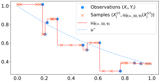
The image is a line chart comparing observations and samples with respect to a variable, likely time or another continuous parameter. It displays three data series: "Observations (Xi, Yi)", "Samples (Xj(r), uθ(∞, 30, 9)(Xj(r)))", and "u*". The chart visualizes how the samples approximate the observations and compares them to a reference line.
### Components/Axes
* **X-axis:** Ranges from 0.0 to 1.0, with increments of 0.2.
* **Y-axis:** Ranges from 0.4 to 1.0, with increments of 0.2.
* **Legend (Top-Right):**
* Blue circle: Observations (Xi, Yi)
* Orange 'x': Samples (Xj(r), uθ(∞, 30, 9)(Xj(r)))
* Red line: uθ(∞, 30, 9)
* Blue dashed line: u*
### Detailed Analysis
* **Observations (Xi, Yi) - Blue Circles:**
* (0, 1.0)
* (0.2, 1.0)
* (0.25, 0.82)
* (0.55, 0.58)
* (0.78, 0.28)
* **Samples (Xj(r), uθ(∞, 30, 9)(Xj(r))) - Orange 'x':**
* The samples form a step-wise function.
* From x=0 to x=0.2, the samples are at y=1.0.
* Around x=0.2, the samples drop to y=0.7.
* From x=0.3 to x=0.4, the samples are at y=0.86.
* From x=0.4 to x=0.6, the samples are at y=0.58.
* From x=0.7 to x=0.8, the samples are at y=0.38.
* From x=0.8 to x=1.0, the samples are at y=0.38.
* **uθ(∞, 30, 9) - Red Line:**
* This line also forms a step-wise function, closely following the samples.
* From x=0 to x=0.2, the line is at y=1.0.
* From x=0.2 to x=0.3, the line drops to y=0.7.
* From x=0.3 to x=0.4, the line rises to y=0.86.
* From x=0.4 to x=0.6, the line drops to y=0.58.
* From x=0.6 to x=0.8, the line drops to y=0.28.
* From x=0.8 to x=1.0, the line rises to y=0.38.
* **u* - Blue Dashed Line:**
* This line is a straight, downward-sloping line.
* At x=0, y=1.0.
* At x=1, y=0.2.
### Key Observations
* The "Samples" and "uθ(∞, 30, 9)" lines are very similar, with the red line connecting the orange 'x' markers.
* The "Observations" are scattered around the "Samples" line.
* The "u*" line is a linear approximation.
### Interpretation
The chart illustrates how the samples (Xj(r), uθ(∞, 30, 9)(Xj(r))) approximate the underlying observations (Xi, Yi). The step-wise function uθ(∞, 30, 9) appears to be a discrete approximation of the observations, while u* represents a linear approximation. The samples are clustered around the step-wise function, indicating that the sampling method is effective in capturing the underlying data distribution. The difference between the observations and the samples represents the error or uncertainty in the approximation.