## Scatter Plot with Step Function and Theoretical Curve
### Overview
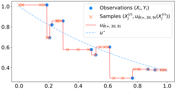
The image is a technical plot comparing observed data points, sampled points, a step-function approximation, and a theoretical curve. It visualizes the relationship between two variables, X and Y, across the unit interval [0, 1]. The plot demonstrates how a set of discrete observations and samples relate to a piecewise constant function and a smooth, decreasing theoretical function.
### Components/Axes
* **Chart Type:** Scatter plot overlaid with step functions and a dashed line.
* **X-Axis:** Linear scale from 0.0 to 1.0, with major tick marks at 0.0, 0.2, 0.4, 0.6, 0.8, and 1.0. No explicit axis label is present.
* **Y-Axis:** Linear scale from approximately 0.3 to 1.0, with major tick marks at 0.4, 0.6, 0.8, and 1.0. No explicit axis label is present.
* **Legend:** Located in the top-right quadrant of the plot area. It contains four entries:
1. **Blue Circle:** `Observations (Xᵢ, Yᵢ)`
2. **Orange 'x' Marker:** `Samples (Xⱼ⁽ʳ⁾, u_θ̂(∞, 30, 9)(Xⱼ⁽ʳ⁾))`
3. **Red Solid Line:** `u_θ̂(∞, 30, 9)`
4. **Blue Dashed Line:** `u*`
* **Plot Area:** Contains all data series and functions described in the legend.
### Detailed Analysis
**1. Observations (Blue Circles):**
These are discrete data points. Their approximate (X, Y) coordinates, reading from left to right, are:
* (0.20, 1.00)
* (0.22, 0.70)
* (0.25, 0.82)
* (0.30, 0.86)
* (0.50, 0.58)
* (0.52, 0.53)
* (0.62, 0.60)
* (0.78, 0.30)
* (0.88, 0.38)
* (0.92, 0.38)
**2. Samples (Orange 'x' Markers):**
These points are clustered around the observations and along the step function. They appear to be generated from or associated with the function `u_θ̂(∞, 30, 9)`. Notable clusters are near X=0.0-0.2 (Y≈1.0), X=0.25-0.30 (Y≈0.85), X=0.50-0.55 (Y≈0.55-0.60), X=0.60-0.65 (Y≈0.60), and X=0.80-1.0 (Y≈0.38).
**3. Step Function `u_θ̂(∞, 30, 9)` (Red Solid Line):**
This is a piecewise constant (step) function. Its value changes at specific X-coordinates, creating horizontal segments connected by vertical jumps.
* **Trend:** The function generally decreases in a stepwise manner from left to right.
* **Key Transitions (Approximate):**
* Starts at Y=1.0 from X=0.0 to X≈0.20.
* Drops vertically to Y≈0.70 at X≈0.20.
* Horizontal at Y≈0.70 until X≈0.22.
* Jumps up to Y≈0.82 at X≈0.22.
* Horizontal at Y≈0.82 until X≈0.25.
* Jumps up to Y≈0.86 at X≈0.25.
* Horizontal at Y≈0.86 until X≈0.30.
* Drops vertically to Y≈0.58 at X≈0.30.
* Horizontal at Y≈0.58 until X≈0.50.
* Drops vertically to Y≈0.53 at X≈0.50.
* Horizontal at Y≈0.53 until X≈0.52.
* Jumps up to Y≈0.60 at X≈0.52.
* Horizontal at Y≈0.60 until X≈0.62.
* Drops vertically to Y≈0.30 at X≈0.62.
* Horizontal at Y≈0.30 until X≈0.78.
* Jumps up to Y≈0.38 at X≈0.78.
* Horizontal at Y≈0.38 from X≈0.78 to X=1.0.
**4. Theoretical Curve `u*` (Blue Dashed Line):**
* **Trend:** A smooth, monotonically decreasing curve.
* **Path:** It starts at (0.0, 1.0) and ends at (1.0, approximately 0.35). It passes below most of the step function's horizontal segments in the first half of the plot and above them in the latter half, intersecting the step function at several points.
### Key Observations
1. **Clustering:** The orange "Samples" are not randomly distributed but are tightly clustered around the blue "Observations" and along the horizontal segments of the red step function.
2. **Step Function Alignment:** The red step function `u_θ̂(∞, 30, 9)` appears to be an approximation derived from the observations. Its horizontal levels often correspond to the Y-values of nearby observation clusters (e.g., the segment at Y≈0.86 aligns with observations at (0.25, 0.82) and (0.30, 0.86)).
3. **Relationship Between Curves:** The smooth blue dashed line `u*` acts as a continuous baseline or target. The red step function approximates it in a piecewise constant manner, with the steps becoming larger and the approximation coarser in regions where `u*` is steeper (e.g., between X=0.3 and X=0.6).
4. **Outlier/Notable Point:** The observation at (0.78, 0.30) is the lowest Y-value and sits directly on a long horizontal segment of the step function, which then jumps up to meet the cluster of samples and observations near Y=0.38.
### Interpretation
This plot likely illustrates a concept from approximation theory, machine learning, or nonparametric statistics. The data suggests the following:
* **Approximation Process:** The red step function `u_θ̂(∞, 30, 9)` is a data-driven, piecewise constant estimator of the unknown true function `u*` (blue dashed line). The estimator is built using a set of observations `(Xᵢ, Yᵢ)`.
* **Role of Samples:** The orange "Samples" `(Xⱼ⁽ʳ⁾, u_θ̂(...)(Xⱼ⁽ʳ⁾))` are likely points used to evaluate or construct the step function estimator. Their clustering indicates regions of interest or high density in the input space (X-axis).
* **Model Behavior:** The estimator captures the general decreasing trend of `u*` but does so with discrete jumps. The quality of the approximation varies; it is closer to `u*` where the data is dense (e.g., near X=0.2 and X=0.5) and deviates more in between. The long horizontal segment from X=0.62 to X=0.78 suggests a region with sparse data, leading the estimator to hold a constant value.
* **Underlying Concept:** The notation `u_θ̂(∞, 30, 9)` hints at a model with parameters `θ̂` possibly related to sample size (30) and another hyperparameter (9). The plot demonstrates how such a model, trained on discrete observations, produces a function that balances fitting the data points and approximating a smoother underlying truth. The tension between the jagged red line and the smooth blue line visually represents the bias-variance tradeoff or the challenge of nonparametric regression.