\n
## Diagram: Signal Timing or Dependency Chart
### Overview
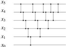
The image displays a technical diagram consisting of six horizontal lines, each labeled on the left side, with a series of vertical lines connecting dots placed at intersections. This structure is characteristic of a timing diagram, signal waveform chart, or a dependency graph commonly used in digital electronics, computer architecture, or systems engineering to illustrate the state transitions or causal relationships between multiple signals or variables over a sequence of events or time.
### Components/Axes
* **Labels (Left Side, Vertically Aligned):**
* `X5` (Topmost line)
* `X4`
* `X3`
* `X2`
* `X1`
* `X0` (Bottommost line)
* **Graphical Elements:**
* Six parallel, horizontal lines extending from the labels to the right edge of the diagram. These represent distinct signals, states, or variables.
* A series of solid black dots placed at specific intersections of the horizontal lines and implied vertical time/event axes.
* Vertical line segments connecting these dots, indicating a relationship, transition, or dependency between the signals at those points.
### Detailed Analysis
The diagram is structured as a grid where the horizontal lines are the primary axes for the signals `X0` through `X5`. The vertical connections define the system's behavior.
**Spatial Layout and Connections (from bottom to top, left to right):**
1. A dot on the `X0` line is connected by a vertical line upward to a dot on the `X1` line.
2. From that dot on `X1`, a vertical line extends upward to a dot on the `X2` line.
3. From the same dot on `X1`, another vertical line extends upward to a dot on the `X3` line.
4. From the dot on `X2` (connected from `X1`), a vertical line extends upward to a dot on the `X3` line.
5. From this dot on `X3` (connected from `X2`), a vertical line extends upward to a dot on the `X4` line.
6. From the same dot on `X3`, another vertical line extends upward to a dot on the `X5` line.
7. From the dot on `X4` (connected from `X3`), a vertical line extends upward to a dot on the `X5` line.
8. Further to the right, a separate vertical line connects a dot on `X4` directly to a dot on `X5`.
9. Even further right, another vertical line connects a dot on `X3` directly to a dot on `X4`.
**Pattern Summary:** The connections form a directed, acyclic graph. Changes or events appear to propagate upward from lower-indexed signals (`X0`, `X1`) to higher-indexed ones (`X4`, `X5`). The structure shows fan-out (e.g., `X1` influences both `X2` and `X3`) and convergence (e.g., `X3` is influenced by both `X1` and `X2`).
### Key Observations
* **Hierarchical Dependency:** There is a clear bottom-up flow of influence. `X0` is the root, affecting `X1`, which then affects multiple higher-level signals.
* **Fan-out and Convergence:** Signal `X1` has a fan-out of 2 (to `X2` and `X3`). Signal `X3` is a point of convergence, receiving inputs from both `X1` and `X2`.
* **Multiple Paths:** There are multiple paths from lower to higher signals (e.g., `X1 -> X3 -> X5` and `X1 -> X2 -> X3 -> X5`).
* **Late-Stage Direct Connection:** The rightmost connections show direct links between `X3`↔`X4` and `X4`↔`X5`, independent of the earlier, more complex branching structure. This could represent a different phase of operation or a separate control path.
* **No Temporal Axis:** The diagram lacks an explicit horizontal time axis. The sequence is implied by the left-to-right arrangement of the vertical connection clusters.
### Interpretation
This diagram is a **dependency or causality graph** for a system with six components or signals (`X0`-`X5`). It visually answers the question: "Which signal's state change triggers or necessitates a change in another signal?"
* **What it Demonstrates:** It maps the propagation of events or data through a system. An initial event at `X0` triggers `X1`. The state of `X1` then becomes a prerequisite for changes in both `X2` and `X3`. The system exhibits both sequential logic (`X1 -> X2 -> X3`) and parallel logic (`X1 -> X3` directly). The final outputs or states `X4` and `X5` depend on a combination of these intermediate signals.
* **Potential Context:** This is typical for illustrating:
* **Digital Circuit Timing:** Showing when control signals must be stable relative to clock edges or other signals.
* **State Machine Transitions:** Depicting how the system moves from one state to another based on inputs.
* **Data Flow in a Pipeline:** Showing how data moves through different processing stages.
* **Fault Propagation Analysis:** Tracing how an error in one component (`X0`) could cascade through the system.
* **Notable Anomaly:** The lack of a labeled time or sequence axis is a significant omission for a pure timing diagram. This suggests the diagram's primary purpose is to show **logical dependency** rather than precise temporal relationships. The spatial left-to-right ordering is a proxy for sequence, but not a calibrated scale.
**In essence, this image provides a structural blueprint of causal relationships within a multi-component system, highlighting its hierarchical and interconnected nature.**