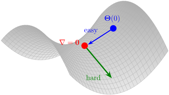
## 3D Surface Plot: Optimization Landscape with Critical Points ### Overview The image depicts a 3D surface plot representing an optimization landscape. A red dot labeled "∇ = 0" marks a saddle point at the center of the surface. Two directional arrows emanate from this point: a blue arrow labeled "easy" pointing toward a blue dot labeled "Θ(0)" (likely a local minimum), and a green arrow labeled "hard" pointing downward into a steeper region of the surface. The surface itself has a grid pattern to indicate curvature and gradient direction. --- ### Components/Axes - **Surface**: A 3D terrain-like plot with a grid overlay, representing the function's topography. - **Red Dot (Center)**: Labeled "∇ = 0", indicating a critical point (saddle point) where the gradient vanishes. - **Blue Arrow ("easy")**: Points from the saddle point to a blue dot labeled "Θ(0)", suggesting a direction of easier descent toward a local minimum. - **Green Arrow ("hard")**: Points downward from the saddle point into a steeper region of the surface, labeled "hard" to denote a more challenging descent path. - **Grid Pattern**: Implicitly encodes curvature and gradient magnitude across the surface. --- ### Detailed Analysis 1. **Saddle Point (∇ = 0)**: - Located at the center of the surface. - Represents a critical point where the gradient is zero but is neither a local minimum nor maximum. - The surface curves upward in one direction (toward the blue dot) and downward in another (toward the green arrow's path). 2. **Blue Arrow ("easy")**: - Color: Blue (matches legend label "easy"). - Direction: Points from the saddle point to the blue dot labeled "Θ(0)". - Implies a path of least resistance toward a local minimum. 3. **Green Arrow ("hard")**: - Color: Green (matches legend label "hard"). - Direction: Points downward from the saddle point into a steeper region. - Indicates a direction of higher gradient magnitude, requiring more computational effort to navigate. 4. **Surface Curvature**: - The grid pattern shows opposing curvatures around the saddle point: - Concave upward toward the blue dot (local minimum). - Concave downward toward the green arrow's path. --- ### Key Observations - The saddle point ("∇ = 0") is a critical point with zero gradient but non-extremal behavior. - The "easy" direction (blue) aligns with a local minimum ("Θ(0)"), suggesting a favorable descent path. - The "hard" direction (green) leads to a steeper region, representing a more challenging optimization trajectory. - The surface's grid confirms the saddle point's mixed curvature properties. --- ### Interpretation This diagram illustrates the challenges of optimization in non-convex landscapes: 1. **Saddle Points as Bottlenecks**: The red dot ("∇ = 0") represents a critical point where gradient-based methods stall, as the gradient vanishes but the point is not a local extremum. 2. **Directional Bias**: The "easy" (blue) and "hard" (green) labels highlight the asymmetry in optimization paths. Algorithms may favor the "easy" direction toward "Θ(0)" but risk getting trapped in suboptimal regions if the "hard" path is not explored. 3. **Curvature Dynamics**: The opposing curvatures around the saddle point emphasize the need for second-order methods (e.g., Hessian-aware optimization) to escape such regions effectively. The visualization underscores the importance of understanding landscape geometry in optimization, particularly for non-convex problems where saddle points and mixed curvature dominate.