TECHNICAL ASSET FINGERPRINT
76708c04aba82808f655eb35
Click to view fullscreen
Press ESC or click to close
FOUND IN PAPERS
EXPERT: healer-alpha-free VERSION 1
RUNTIME: free/openrouter/healer-alpha
INTEL_VERIFIED
## Technical Diagram: Transformer Layer Architecture with Parallel Attention and MLP Blocks
### Overview
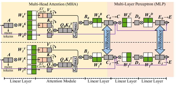
This image is a technical schematic diagram illustrating the internal architecture of a transformer-based neural network layer. It specifically depicts a parallelized design where the Multi-Head Attention (MHA) and Multi-Layer Perceptron (MLP) computations are processed concurrently, likely across different devices or cores, as indicated by the "AllReduce" communication operations. The diagram uses a flowchart style with boxes representing data tensors or matrices, circles with crosses representing matrix multiplication operations, and arrows indicating data flow.
### Components/Axes
The diagram is divided into two primary horizontal sections, separated by a dashed line, representing two parallel processing streams (e.g., for two different devices or model shards).
**1. Top Section (Stream 0):**
* **Header Label:** "Multi-Head Attention (MHA)" on the left, "Multi-Layer Perceptron (MLP)" on the right.
* **Input:** A gray box labeled **`A`** (input activations). An arrow points from it with the text "more tokens".
* **MHA Block:**
* Three parallel branches for Query (Q), Key (K), and Value (V) projections.
* **Weight Matrices (Green):** `W_0^K`, `W_0^V`, `W_0^Q`.
* **Projected Tensors (Gray):** `K_0`, `V_0`, `Q_0`.
* **KV Cache:** A pink box labeled "KV Cache" is associated with `K_0` and `V_0`.
* **Attention Operation:** `Q_0` and `K_0` are multiplied (`Q_0 K_0^T`), followed by a **`Softmax`** operation (vertical gray box). The result is multiplied with `V_0`.
* **Output Tensor (Gray):** `B_0`.
* **MLP Block:**
* **First Linear Layer:** `B_0` is multiplied by a green weight matrix `W_0^B`, resulting in tensor `C_0`.
* **AllReduce Operation:** A large, double-headed blue arrow labeled **`AllReduce`** connects `C_0` in the top stream to `C_1` in the bottom stream, indicating a synchronization/communication step.
* **Second Linear Layer:** The synchronized `C_0` is multiplied by green weight matrix `W_0^C`, resulting in tensor `D_0`.
* **Third Linear Layer:** `D_0` is multiplied by green weight matrix `W_0^D`, resulting in tensor `E_0`.
* **Output:** The final tensor is labeled **`E`**.
**2. Bottom Section (Stream 1):**
* This section is structurally identical to the top section, with all subscript indices changed from `0` to `1`.
* **Weight Matrices:** `W_1^K`, `W_1^V`, `W_1^Q`, `W_1^B`, `W_1^C`, `W_1^D`.
* **Tensors:** `A`, `K_1`, `V_1`, `Q_1`, `B_1`, `C_1`, `D_1`, `E_1`, `E`.
* **Operations:** Identical matrix multiplications and `Softmax`.
* **AllReceive Operation:** The same blue `AllReduce` arrow connects `C_1` to `C_0`.
**3. Footer Labels (Bottom of Diagram):**
A series of labels aligned with the processing stages from left to right:
* `Linear Layer` (under the initial projection from `A`)
* `Attention Module` (under the QKV operations)
* `Linear Layer` (under the `W_0^B`/`W_1^B` multiplication)
* `Linear Layer` (under the `W_0^C`/`W_1^C` multiplication)
* `Linear Layer` (under the `W_0^D`/`W_1^D` multiplication)
### Detailed Analysis
* **Data Flow & Parallelism:** The diagram explicitly shows a model parallelism strategy. The input `A` is duplicated to both streams. The MHA and initial MLP linear layer (`W^B`) are computed independently on each stream. The critical synchronization point is the `AllReduce` operation on the intermediate tensor `C` (output of the first MLP linear layer). This operation likely sums or averages the `C_0` and `C_1` tensors across streams before proceeding to the subsequent MLP layers (`W^C`, `W^D`). The final output `E` is also shown as a single entity, suggesting it is gathered or replicated after the final computation.
* **KV Cache:** The presence of the "KV Cache" label next to `K_0` and `V_0` (and `K_1`, `V_1`) indicates this architecture is optimized for autoregressive inference, where previously computed Key and Value vectors are stored to avoid recomputation.
* **Matrix Dimensions (Inferred):** The green weight matrices (`W`) are depicted as rectangular blocks, suggesting they are 2D matrices. The gray tensor boxes (`A`, `B`, `C`, etc.) are also rectangular, implying they are 2D tensors (e.g., [sequence_length, hidden_dimension]). The `Q K^T` operation results in a square-like box, consistent with an attention score matrix of shape [seq_len, seq_len].
* **Color Coding:**
* **Green:** Trainable weight matrices/parameters.
* **Gray:** Data activations/tensors and core operations (Softmax).
* **Blue:** Communication operation (AllReduce).
* **Pink:** Cached data (KV Cache).
### Key Observations
1. **Symmetrical Parallel Design:** The two streams are perfect mirrors, indicating a balanced split of the model's hidden dimension or attention heads across two processing units.
2. **Synchronization Point:** The `AllReduce` is placed after the first linear transformation in the MLP block. This is a specific design choice for pipeline or tensor parallelism, ensuring the streams have the same data before the final nonlinear transformations.
3. **No Residual Connections Shown:** The diagram focuses on the core computational blocks (Attention and MLP) and their parallelization. Standard transformer residual connections (add & norm) are not depicted in this specific schematic.
4. **Linear Layer Proliferation:** The MLP is explicitly broken down into three sequential linear layers (`W^B`, `W^C`, `W^D`), which is a more granular view than the typical "two linear layers with an activation in between" description. This may represent a specific implementation or a more detailed breakdown of a single feed-forward block.
### Interpretation
This diagram provides a detailed, low-level view of a **distributed transformer inference engine**. It answers the question: "How is a single transformer layer split and executed across multiple devices to reduce memory footprint and/or increase speed?"
The key insight is the **interleaving of computation and communication**. The devices work independently on their portions of the attention and the first part of the MLP. They must then synchronize (`AllReduce`) to combine their partial results before completing the MLP computation. This pattern is characteristic of **tensor parallelism** (specifically, splitting the MLP layer's hidden dimension).
The inclusion of the "KV Cache" label strongly suggests this architecture is designed for **efficient autoregressive generation** (e.g., for large language models), where minimizing latency and memory bandwidth is critical. The parallelization helps manage the large memory requirement of both the model weights and the growing KV cache for long sequences.
**Notable Anomaly/Design Choice:** The placement of the `AllReduce` *within* the MLP block, rather than after the entire Attention+MLP layer, is significant. It implies that the MLP's first linear layer (`W^B`) is sharded, and its output must be aggregated before the subsequent non-linearity and final linear layers. This is a more communication-intensive but potentially more memory-efficient strategy than other parallelism schemes.
DECODING INTELLIGENCE...