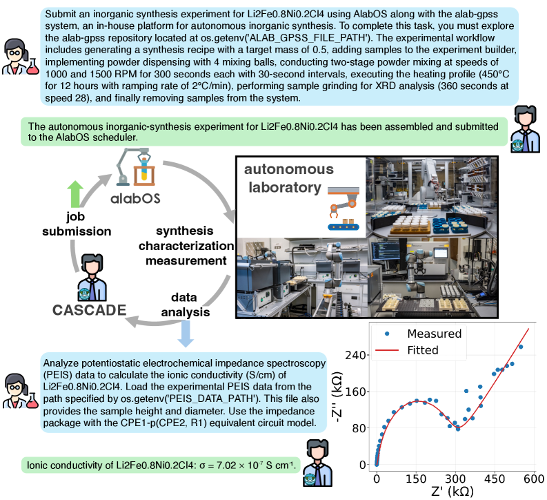
## Technical Document: Inorganic Synthesis Experiment Workflow and Data Analysis ### Overview The image depicts a technical workflow for an autonomous inorganic synthesis experiment using the AlabOS platform and alab-gpss repository. It includes a flowchart of the experimental process, a graph of electrochemical impedance spectroscopy (EIS) data, and descriptions of laboratory automation. Key elements include synthesis parameters, data analysis steps, and a plot of ionic conductivity. --- ### Components/Axes #### Text Blocks 1. **Experiment Submission Instructions**: - Target: Li2Fe0.8Ni0.2Cl4 synthesis - Workflow: - Generate synthesis recipe with 0.5g target mass - Implement powder dispensing (4 mixing balls, 1000/1500 RPM, 300s each) - Two-stage mixing at 450°C (30s intervals, 12h total) - Sample grinding for XRD (360s at 28°C/min) - Sample removal - Submission status: "The autonomous inorganic-synthesis experiment for Li2Fe0.8Ni0.2Cl4 has been assembled and submitted to the AlabOS scheduler." 2. **Data Analysis Instructions**: - Analyze PEIS data to calculate ionic conductivity (S/cm) - Load experimental PEIS data from `os.getenv('PEIS_DATA_PATH')` - Use impedance package with CPE1-p(CPE2, R1) equivalent circuit model - Result: Ionic conductivity of Li2Fe0.8Ni0.2Cl4: σ = 7.02×10⁻⁷ S/cm #### Diagram (Flowchart) - **Components**: - Job submission (human icon) - AlabOS platform (central node) - Synthesis (flask icon) - Characterization (microscope icon) - Measurement (spectrometer icon) - Data analysis (computer icon) - Cascade system (loop arrow) - **Flow**: - Job submission → AlabOS → Synthesis → Characterization → Measurement → Data analysis → Cascade #### Graph (EIS Data) - **Axes**: - X-axis: Z' (kΩ) [0–600] - Y-axis: -Z'' (kΩ) [0–240] - **Legend**: - Blue dots: Measured data - Red line: Fitted curve - **Key Data Point**: - Ionic conductivity: σ = 7.02×10⁻⁷ S/cm (annotated in text) #### Laboratory Image - **Components**: - Robotic arms (blue/gray) - Sample holders (yellow/orange) - Automated equipment (conveyors, grinders) - Control panels (monitors, buttons) --- ### Detailed Analysis #### Text Blocks - **Synthesis Parameters**: - Target mass: 0.5g - Mixing: 4 balls, 1000/1500 RPM, 300s per stage - Temperature: 450°C (30s intervals, 12h total) - Grinding: 360s at 28°C/min ramping - **Data Analysis**: - PEIS data path: `os.getenv('PEIS_DATA_PATH')` - Sample dimensions: Height/diameter provided - Circuit model: CPE1-p(CPE2, R1) #### Graph - **Trend**: - Measured data (blue dots) shows a U-shaped curve with a minimum at ~200 kΩ - Fitted curve (red line) closely follows the data, with slight deviations - **Key Observation**: - Ionic conductivity (σ) derived from EIS data: 7.02×10⁻⁷ S/cm --- ### Key Observations 1. The synthesis workflow emphasizes precision (e.g., 30s intervals, 2°C/min ramping). 2. The EIS graph shows a typical semicircular arc, indicating charge transfer resistance and diffusion processes. 3. The ionic conductivity value (7.02×10⁻⁷ S/cm) suggests moderate ionic mobility in the synthesized material. --- ### Interpretation - **Workflow Integration**: The AlabOS platform automates synthesis and data collection, reducing human intervention. The Cascade system ensures iterative refinement. - **Material Properties**: The ionic conductivity value (7.02×10⁻⁷ S/cm) indicates the material’s potential for applications requiring ion transport (e.g., batteries, sensors). - **Data Validation**: The close match between measured and fitted EIS data validates the equivalent circuit model (CPE1-p(CPE2, R1)). - **Automation Impact**: Robotic systems (e.g., powder dispensing, sample grinding) enable reproducibility and scalability of experiments. --- ### Notable Trends - The EIS curve’s minimum at ~200 kΩ suggests optimal ionic conductivity at this frequency. - The synthesis parameters (high temperature, prolonged mixing) likely enhance material homogeneity, reflected in the conductivity data.