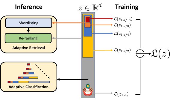
## System Architecture Diagram: Adaptive Retrieval and Classification via Latent Vector Segmentation ### Overview This image is a technical system architecture diagram illustrating a machine learning framework that uses a shared latent vector representation for multiple hierarchical tasks. The diagram is divided into two primary sections: **Inference** (left) and **Training** (right), connected by a central latent vector \( z \in \mathbb{R}^d \). The system appears to employ a form of multi-task or hierarchical learning where different segments of the latent vector are optimized for and utilized by specific sub-tasks. ### Components/Axes The diagram is organized into three main spatial regions: 1. **Left Region (Inference):** Contains two primary modules. * **Top Module:** Labeled "Adaptive Retrieval" (beige box). Inside, it contains two sequential sub-components: "Shortlisting" (light blue box) and "Re-ranking" (green box). * **Bottom Module:** Labeled "Adaptive Classification" (beige box). It contains a visual representation of a hierarchical or multi-scale classification process, depicted as a series of colored bars (red, orange, blue, yellow) with a dashed arrow pointing from a smaller set of bars to a larger, more detailed set. 2. **Central Region (Latent Representation):** * A vertical gray bar represents the latent vector \( z \), with the mathematical notation \( z \in \mathbb{R}^d \) placed above it. * The vector is segmented into colored blocks of varying lengths. From top to bottom, the visible colors are: **red** (shortest), **orange**, **blue**, and **yellow** (longest). These segments are nested, with the red segment contained within the orange, which is within the blue, which is within the yellow, suggesting a hierarchical or progressive structure. 3. **Right Region (Training):** * Labeled "Training" at the top. * Shows a series of loss functions, each connected by an arrow to a specific colored segment of the central vector \( z \). * The loss functions are: \( \mathcal{L}(z_{1:d/16}) \) (red arrow), \( \mathcal{L}(z_{1:d/8}) \) (orange arrow), \( \mathcal{L}(z_{1:d/4}) \) (blue arrow), and \( \mathcal{L}(z_{1:d/2}) \) (yellow arrow). * These individual losses are summed (indicated by a circled plus symbol ⊕) to form a total loss, \( \mathcal{L}(z) \). * At the bottom of the vector, a final loss \( \mathcal{L}(z_{1:d}) \) is shown, connected to an icon of a red pot with a green plant sprouting from it, symbolizing the full vector or a foundational task. ### Detailed Analysis **Flow and Relationships:** * **Training Flow (Right to Center):** During training, the system computes multiple loss functions on progressively larger segments of the latent vector \( z \). The notation \( z_{1:d/n} \) suggests the loss is calculated on the first \( d/n \) dimensions of the vector. The losses are hierarchical: \( \mathcal{L}(z_{1:d/16}) \) acts on the smallest (red) segment, \( \mathcal{L}(z_{1:d/8}) \) on the red+orange segments, and so on, culminating in \( \mathcal{L}(z_{1:d}) \) on the entire vector. These are combined into a single total loss \( \mathcal{L}(z) \). * **Inference Flow (Center to Left):** During inference, the trained latent vector \( z \) is used by different modules. * The top segments (red, orange, blue) are routed to the **Adaptive Retrieval** module. An orange arrow points from the orange segment to "Shortlisting," and a gray arrow points from the blue segment to "Re-ranking." This suggests the shorter, more abstract segments of the vector are used for coarse retrieval (shortlisting), while slightly longer segments are used for finer re-ranking. * The longest segment (yellow) is routed to the **Adaptive Classification** module, as indicated by a black arrow. The visual inside this module shows the colored bars expanding, implying that classification uses the most detailed part of the representation. **Color-Coding Consistency:** * **Red Segment:** Linked to loss \( \mathcal{L}(z_{1:d/16}) \). No direct inference arrow is shown, but it is the core of the hierarchy. * **Orange Segment:** Linked to loss \( \mathcal{L}(z_{1:d/8}) \). Connected via an orange arrow to the "Shortlisting" component in Adaptive Retrieval. * **Blue Segment:** Linked to loss \( \mathcal{L}(z_{1:d/4}) \). Connected via a gray arrow to the "Re-ranking" component in Adaptive Retrieval. * **Yellow Segment:** Linked to loss \( \mathcal{L}(z_{1:d/2}) \). Connected via a black arrow to the "Adaptive Classification" module. * **Full Vector (Pot Icon):** Linked to loss \( \mathcal{L}(z_{1:d}) \). ### Key Observations 1. **Hierarchical Latent Space:** The core innovation is the explicit segmentation of the latent vector \( z \) into a hierarchy of subspaces (1/16, 1/8, 1/4, 1/2, full), each associated with a specific loss function during training. 2. **Task-Specific Routing:** Different segments of the same vector are allocated to different inference tasks (retrieval vs. classification), promoting efficiency and specialization within a shared representation. 3. **Multi-Scale Training Objective:** The total loss \( \mathcal{L}(z) \) is a sum of losses computed at different scales of the representation, which likely encourages the model to learn features useful at multiple levels of abstraction. 4. **Visual Metaphor:** The "plant in a pot" icon at the bottom likely symbolizes the foundational or "root" representation from which other tasks grow, or it may represent a base task (like auto-encoding) that uses the full vector. ### Interpretation This diagram outlines a framework for **efficient multi-task learning**. The key idea is to train a single, structured latent representation where different portions of the vector are explicitly optimized for different downstream tasks of varying complexity. * **What it suggests:** The system learns a compressed, hierarchical knowledge base. Coarse, high-level information (stored in the top segments) is sufficient for fast, approximate tasks like retrieval shortlisting. Finer-grained information (stored in the lower segments) is required for more precise tasks like re-ranking and detailed classification. This mimics human cognition, where we might quickly recall a category before accessing specific details. * **How elements relate:** The training process (right) shapes the latent space \( z \) by applying pressure at multiple scales. This directly determines how the space is partitioned and utilized during inference (left). The architecture enforces a separation of concerns within a unified model. * **Notable implications:** This approach could lead to significant computational savings during inference, as the full vector need not be processed for every task. It also provides interpretability, as one can analyze which vector segments are important for which tasks. The primary challenge would be balancing the multiple loss terms during training to ensure all segments learn meaningful features without interfering with each other. The diagram presents a clean, theoretical model; its practical effectiveness would depend on the specific tasks, data, and implementation details not shown here.