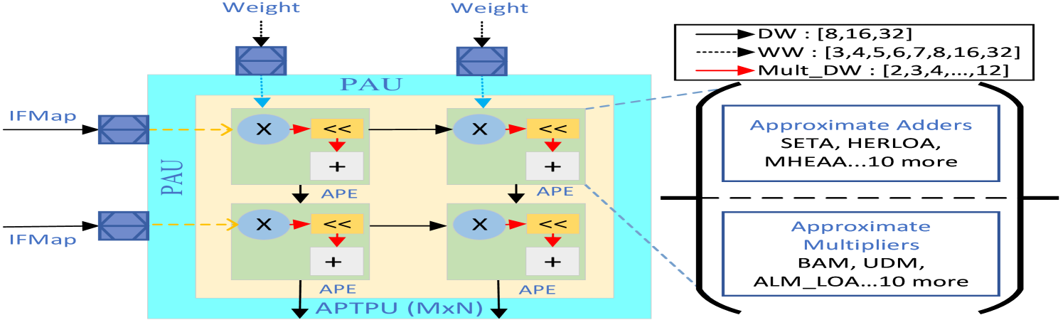
\n ## Diagram: Approximate Processing Unit (APU) Architecture ### Overview The image depicts the architecture of an Approximate Processing Unit (APU), highlighting the flow of Input Feature Maps (IFMap) through Processing Array Units (PAU) and the use of approximate adders and multipliers. The diagram illustrates a parallel processing structure with weight application, multiplication, and accumulation operations. ### Components/Axes The diagram consists of the following key components: * **IFMap:** Input Feature Map – the input data stream. * **Weight:** Input weights applied to the IFMap. * **PAU:** Processing Array Unit – the core processing block. * **APE:** Approximate Processing Element. * **APTPU (MxN):** Approximate Processing Tile Processing Unit – the output of the PAU array. * **Arrows:** Indicate data flow direction. * **Legend (Top-Right):** * Solid Black Arrow: DW : \[8,16,32] * Dashed Black Arrow: WW : \[3,4,5,6,7,8,16,32] * Solid Red Arrow: Mult\_DW : \[2,3,4,...,12] * **Approximate Adders (Bottom-Right):** Listed algorithms: SETA, HERLOA, MHEAA…10 more. * **Approximate Multipliers (Bottom-Right):** Listed algorithms: BAM, UDM, ALM\_LOA…10 more. ### Detailed Analysis or Content Details The diagram shows two parallel processing paths. Each path consists of the following stages: 1. **Input:** An IFMap enters the PAU. 2. **Weight Application:** A Weight is applied to the IFMap. 3. **Multiplication:** The weighted IFMap is multiplied (indicated by the 'X' symbol) using approximate multipliers (represented by the red arrows labeled "Mult\_DW : \[2,3,4,...,12]"). 4. **Shift Operation:** A right shift operation is performed (indicated by the "<<"). 5. **Addition:** The shifted result is added (indicated by the '+' symbol) using approximate adders. 6. **Output:** The final result is output from the APTPU (MxN). The PAU is represented by a light blue square, and there are two PAUs shown in parallel. The dashed cyan arrows represent data flow with a width of "WW : \[3,4,5,6,7,8,16,32]". The solid black arrows represent data flow with a width of "DW : \[8,16,32]". The bottom-right section lists approximate adders and multipliers used in the APU. The approximate adders include SETA, HERLOA, and MHEAA, with "10 more" algorithms not explicitly listed. The approximate multipliers include BAM, UDM, and ALM\_LOA, with "10 more" algorithms not explicitly listed. ### Key Observations * The diagram emphasizes the use of approximate computing techniques (approximate adders and multipliers) to potentially reduce power consumption and improve performance. * The parallel structure of the PAUs suggests a high degree of parallelism in the processing. * The legend indicates different data widths (DW, WW) and multiplication factors (Mult\_DW) used in the processing. * The diagram does not provide specific numerical values for the weights or IFMap data. ### Interpretation The diagram illustrates a hardware architecture designed for efficient approximate computation. The use of PAUs and parallel processing suggests a focus on throughput. The inclusion of approximate adders and multipliers indicates a trade-off between accuracy and efficiency. The different data widths (DW, WW) and multiplication factors (Mult\_DW) suggest a configurable architecture that can be optimized for different applications. The listing of multiple approximate algorithms (SETA, HERLOA, BAM, UDM, etc.) implies a flexible design that can leverage various approximation techniques. The diagram is a high-level representation and does not provide details on the specific implementation of the approximate algorithms or the control logic of the PAUs. The diagram suggests a system designed for applications where some loss of accuracy is acceptable in exchange for significant gains in performance and energy efficiency, such as image processing, machine learning, or signal processing.