## Partial Dependence Plots: Feature Analysis
### Overview
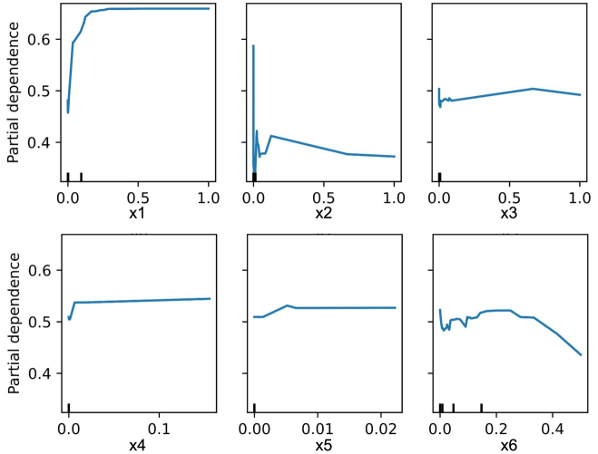
The image presents six partial dependence plots, each illustrating the relationship between a single feature (x1 through x6) and the model's predicted outcome. Each plot shows how the model's prediction changes as the feature value varies, while all other features are held constant.
### Components/Axes
* **Y-axis (Vertical):** "Partial dependence", ranging from approximately 0.4 to 0.7.
* **X-axis (Horizontal):** Feature values for x1, x2, x3, x4, x5, and x6. The ranges vary for each feature:
* x1: 0.0 to 1.0
* x2: 0.0 to 1.0
* x3: 0.0 to 1.0
* x4: 0.0 to 0.1
* x5: 0.00 to 0.02
* x6: 0.0 to 0.4
* **Data Series:** Each plot contains a single blue line representing the partial dependence of the model's prediction on the respective feature.
* **Tick Marks:** Small vertical black lines along the x-axis indicate the distribution of the feature values in the dataset.
### Detailed Analysis
**Plot 1: x1**
* **Trend:** The partial dependence increases sharply from x1 = 0.0 to approximately x1 = 0.2, then plateaus around a partial dependence of 0.7 for x1 values between 0.2 and 1.0.
* **Values:**
* At x1 = 0.0, partial dependence is approximately 0.45.
* At x1 = 0.2, partial dependence reaches approximately 0.7.
* From x1 = 0.2 to 1.0, partial dependence remains roughly constant at 0.7.
**Plot 2: x2**
* **Trend:** The partial dependence shows a sharp spike near x2 = 0.0, followed by a rapid decrease, and then a gradual decline as x2 increases.
* **Values:**
* At x2 = 0.0, partial dependence peaks at approximately 0.6.
* At x2 = 0.1, partial dependence drops to approximately 0.4.
* At x2 = 1.0, partial dependence is approximately 0.3.
**Plot 3: x3**
* **Trend:** The partial dependence starts with a sharp increase near x3 = 0.0, followed by a slight increase until x3 = 0.6, and then a slight decrease until x3 = 1.0.
* **Values:**
* At x3 = 0.0, partial dependence is approximately 0.48.
* At x3 = 0.6, partial dependence reaches approximately 0.5.
* At x3 = 1.0, partial dependence decreases to approximately 0.49.
**Plot 4: x4**
* **Trend:** The partial dependence increases sharply from x4 = 0.0 to approximately x4 = 0.01, then plateaus around a partial dependence of 0.54 for x4 values between 0.01 and 0.1.
* **Values:**
* At x4 = 0.0, partial dependence is approximately 0.5.
* At x4 = 0.01, partial dependence reaches approximately 0.54.
* From x4 = 0.01 to 0.1, partial dependence remains roughly constant at 0.54.
**Plot 5: x5**
* **Trend:** The partial dependence increases sharply from x5 = 0.00 to approximately x5 = 0.002, then plateaus around a partial dependence of 0.52 for x5 values between 0.002 and 0.02.
* **Values:**
* At x5 = 0.00, partial dependence is approximately 0.5.
* At x5 = 0.002, partial dependence reaches approximately 0.52.
* From x5 = 0.002 to 0.02, partial dependence remains roughly constant at 0.52.
**Plot 6: x6**
* **Trend:** The partial dependence shows a complex pattern with multiple peaks and valleys. It increases sharply near x6 = 0.0, then decreases, increases again, and finally decreases as x6 approaches 0.4.
* **Values:**
* At x6 = 0.0, partial dependence is approximately 0.5.
* At x6 = 0.1, partial dependence reaches approximately 0.53.
* At x6 = 0.25, partial dependence peaks at approximately 0.53.
* At x6 = 0.4, partial dependence decreases to approximately 0.43.
### Key Observations
* Features x1 and x4 exhibit a strong positive impact on the model's prediction up to a certain threshold, after which the effect plateaus.
* Feature x2 has a strong negative impact on the model's prediction as its value increases.
* Feature x6 has a more complex relationship with the model's prediction, showing non-linear behavior.
* The tick marks on the x-axis indicate the distribution of the feature values. Denser tick marks suggest a higher concentration of data points in that region.
### Interpretation
The partial dependence plots provide insights into how each feature influences the model's predictions. They help understand the marginal effect of each feature, holding all other features constant. This information can be used for:
* **Feature Importance:** Identifying the most influential features in the model.
* **Model Understanding:** Gaining insights into the model's behavior and how it makes predictions.
* **Feature Engineering:** Guiding feature engineering efforts by identifying non-linear relationships and potential interactions between features.
* **Model Debugging:** Identifying potential issues with the model, such as unexpected behavior or biases.
For example, the plot for x1 suggests that increasing x1 up to a value of 0.2 significantly increases the model's prediction, but further increases have little effect. This could indicate a saturation effect or a non-linear relationship that the model has learned. Similarly, the plot for x2 suggests that increasing x2 has a negative impact on the model's prediction. The complex behavior of x6 suggests that it may interact with other features or have a non-linear relationship with the target variable.