## [Chart Type]: Partial Dependence Plots (2x3 Grid)
### Overview
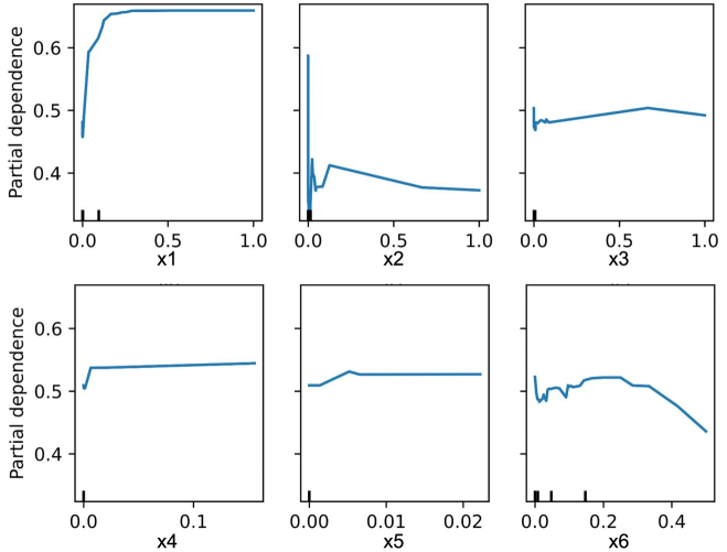
The image displays a set of six individual line charts arranged in a 2-row by 3-column grid. Each chart illustrates the **partial dependence** of a machine learning model's prediction on a single input feature (labeled x1 through x6). Partial dependence plots show the marginal effect of a feature on the predicted outcome, averaging out the effects of all other features. The y-axis is consistent across all plots, while the x-axis scales differ significantly between features.
### Components/Axes
* **Overall Structure:** Six subplots in a 2x3 grid.
* **Y-Axis (All Plots):**
* **Label:** "Partial dependence"
* **Scale:** Linear, ranging from approximately 0.4 to 0.65 (ticks at 0.4, 0.5, 0.6).
* **X-Axes (Individual Plots):**
* **Top Row (Left to Right):**
* **Plot 1:** Label "x1", Scale: 0.0 to 1.0 (ticks at 0.0, 0.5, 1.0).
* **Plot 2:** Label "x2", Scale: 0.0 to 1.0 (ticks at 0.0, 0.5, 1.0).
* **Plot 3:** Label "x3", Scale: 0.0 to 1.0 (ticks at 0.0, 0.5, 1.0).
* **Bottom Row (Left to Right):**
* **Plot 4:** Label "x4", Scale: 0.0 to 0.1 (ticks at 0.0, 0.1).
* **Plot 5:** Label "x5", Scale: 0.00 to 0.02 (ticks at 0.00, 0.01, 0.02).
* **Plot 6:** Label "x6", Scale: 0.0 to 0.4 (ticks at 0.0, 0.2, 0.4).
* **Data Series:** Each plot contains a single blue line representing the partial dependence function for that feature.
* **Additional Markings:** Small vertical tick marks (rug plot) are present along the bottom of each x-axis, indicating the distribution of the feature values in the underlying dataset. The density of these marks is highest near zero for all features.
### Detailed Analysis
**Trend Verification & Data Point Extraction (Approximate):**
1. **Feature x1:**
* **Trend:** Sharp, concave-down increase followed by a plateau.
* **Key Points:** Starts at ~0.45 (x1=0). Rises steeply to ~0.65 by x1≈0.1. Plateaus at ~0.65 from x1≈0.2 to x1=1.0.
2. **Feature x2:**
* **Trend:** Volatile with a sharp initial drop, a mid-range spike, and a gradual decline.
* **Key Points:** Starts high at ~0.60 (x2=0). Drops sharply to a local minimum of ~0.38 at x2≈0.02. Spikes to a peak of ~0.42 at x2≈0.1. Gradually declines to ~0.38 at x2=1.0.
3. **Feature x3:**
* **Trend:** Nearly flat with very minor fluctuations.
* **Key Points:** Hovers consistently around ~0.48 to 0.50 across the entire range (x3=0 to 1.0).
4. **Feature x4:**
* **Trend:** Initial sharp increase followed by a very flat plateau.
* **Key Points:** Starts at ~0.50 (x4=0). Increases rapidly to ~0.54 by x4≈0.01. Remains almost perfectly flat at ~0.54 up to x4=0.1.
5. **Feature x5:**
* **Trend:** Slight initial increase followed by a flat plateau.
* **Key Points:** Starts at ~0.51 (x5=0). Increases gently to ~0.53 by x5≈0.005. Plateaus at ~0.53 up to x5=0.02.
6. **Feature x6:**
* **Trend:** Initial volatility, a broad peak, followed by a clear downward trend.
* **Key Points:** Starts at ~0.52 (x6=0). Shows minor fluctuations, then rises to a broad peak of ~0.53 between x6≈0.1 and 0.2. Declines steadily thereafter, reaching ~0.44 at x6=0.4.
### Key Observations
* **Variable Impact:** Features have vastly different relationships with the model's output. x1 has a strong, saturating positive effect. x2 has a complex, non-monotonic relationship. x3 has almost no effect. x4 and x5 have mild, saturating positive effects over very small value ranges. x6 has a negative effect at higher values.
* **Scale Disparity:** The x-axes for x4, x5, and x6 are orders of magnitude smaller than for x1, x2, and x3. This suggests these features operate on different scales or represent different types of variables (e.g., probabilities vs. counts).
* **Data Distribution:** The rug plots show that for all features, the data is heavily concentrated near zero, with sparse observations at higher values. This is especially pronounced for x4, x5, and x6.
* **Saturation:** The curves for x1, x4, and x5 show clear saturation, where increasing the feature beyond a certain point has no further effect on the prediction.
### Interpretation
This set of partial dependence plots provides a diagnostic view into a model's behavior. It reveals how the model *learns* to use each feature:
* **Feature Importance & Function:** x1 is likely a primary driver of the prediction, with a strong positive influence that caps out. x2's complex curve suggests the model captures a nuanced, possibly interaction-driven relationship. x3 is effectively ignored by the model within the observed data range.
* **Operational Ranges:** The model's sensitivity to x4, x5, and x6 is confined to very low numerical values. This could indicate these are rare-event indicators or normalized features where only small deviations from zero are meaningful.
* **Model Reliability Caution:** The trends for x2 and x6, especially the volatility and decline, are estimated in regions with sparse data (few rug marks). These parts of the curve are less reliable and should be interpreted with caution, as they are extrapolations by the model.
* **Actionable Insight:** If this were a model for, say, customer churn, one might conclude that increasing feature x1 (e.g., "usage frequency") is beneficial up to a point, while high values of x6 (e.g., "support tickets") are detrimental. Feature x3 (e.g., "account age") may not be a useful predictor.
In summary, the plots move beyond simple feature importance scores to show the *direction*, *shape*, and *magnitude* of each feature's influence, which is critical for model understanding, validation, and decision-making.