## Training Loss Curve: Negative Log-Likelihood Loss vs. Epoch
### Overview
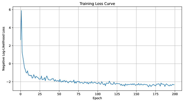
The image displays a line chart titled "Training Loss Curve," plotting the Negative Log-Likelihood Loss of a machine learning model against the number of training epochs. The chart shows a classic convergence pattern, with a rapid initial decrease in loss followed by a gradual stabilization.
### Components/Axes
* **Chart Title:** "Training Loss Curve" (centered at the top).
* **X-Axis:**
* **Label:** "Epoch"
* **Scale:** Linear, ranging from 0 to 200.
* **Major Tick Marks:** At intervals of 25 (0, 25, 50, 75, 100, 125, 150, 175, 200).
* **Y-Axis:**
* **Label:** "Negative Log-Likelihood Loss"
* **Scale:** Linear, ranging from approximately -2 to 6.
* **Major Tick Marks:** At intervals of 2 (-2, 0, 2, 4, 6).
* **Data Series:** A single, solid blue line representing the loss value at each epoch.
* **Grid:** A light gray grid is present, with lines aligned to the major tick marks on both axes.
* **Legend:** None present (single data series).
### Detailed Analysis
The data series exhibits two distinct phases:
1. **Phase 1 - Rapid Descent (Epochs 0 to ~10):**
* **Trend:** The line slopes steeply downward.
* **Data Points (Approximate):**
* Epoch 0: Loss ≈ 6.0
* Epoch 5: Loss ≈ 0.0
* Epoch 10: Loss ≈ -1.0
2. **Phase 2 - Gradual Convergence & Plateau (Epochs ~10 to 200):**
* **Trend:** The line continues to slope downward but at a much shallower angle, eventually flattening into a noisy plateau.
* **Data Points (Approximate):**
* Epoch 25: Loss ≈ -1.8
* Epoch 50: Loss ≈ -2.0
* Epoch 100: Loss ≈ -2.2
* Epoch 150: Loss ≈ -2.4
* Epoch 200: Loss ≈ -2.5
* **Noise:** From approximately epoch 25 onward, the line exhibits consistent, small-scale fluctuations (noise) around the general downward trend. The amplitude of this noise appears relatively constant.
### Key Observations
* **Convergence:** The model's loss converges to a stable value, indicating successful training.
* **Learning Rate:** The extremely steep initial drop suggests a high initial learning rate or a model that quickly learns the most salient features of the data.
* **Plateau Value:** The loss stabilizes at a negative value (≈ -2.5). This is mathematically valid for Negative Log-Likelihood (NLL) loss, as NLL can be negative when the model assigns a probability greater than 1 to the correct class (which is possible in unnormalized log-space calculations).
* **Noise:** The persistent noise in the later epochs is typical of stochastic gradient descent (SGD) or its variants, reflecting updates from mini-batches of data.
### Interpretation
This curve demonstrates a healthy and typical training progression for a probabilistic model (e.g., a classifier using cross-entropy loss). The data suggests:
1. **Effective Learning:** The model rapidly absorbed the primary patterns in the training data within the first 10-20 epochs.
2. **Fine-Tuning:** The subsequent 180 epochs were spent on fine-tuning, where the model made smaller adjustments to its parameters, leading to a slower but continued improvement in fit.
3. **Stability:** The plateau indicates the model has likely reached a local minimum in the loss landscape for the given hyperparameters (learning rate, optimizer). Further training beyond 200 epochs is unlikely to yield significant improvement.
4. **Potential for Optimization:** The presence of noise suggests the learning rate might be slightly high for the later stages of training. A learning rate scheduler that reduces the rate after the initial drop could potentially lead to a smoother convergence to a slightly lower loss value.
**In summary, the chart provides clear visual evidence of a model that has successfully learned from its training data, transitioning from a phase of rapid acquisition of knowledge to one of refinement and stabilization.**