## [Diagram]: Three-Step Process for Interpretable Machine Learning
### Overview
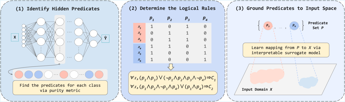
The image is a technical diagram illustrating a three-step methodological pipeline for extracting interpretable logical rules from a neural network. The process flows from left to right across three distinct panels, each enclosed in a dashed blue box. The overall goal is to move from a black-box model (a neural network) to human-understandable logical predicates grounded in the input data space.
### Components/Axes
The diagram is divided into three sequential panels, labeled (1), (2), and (3).
**Panel (1): Identify Hidden Predicates**
* **Visual Component:** A schematic of a feedforward neural network. It has an input layer labeled **X**, multiple hidden layers (represented by circles and connecting lines), and an output layer labeled **Ŷ**.
* **Textual Elements:**
* Title: `(1) Identify Hidden Predicates`
* A yellow text box at the bottom: `Find the predicates for each class via purity metric`.
* Below the network, a sequence of colored circles (red, blue, white) represents data points or class assignments.
* **Spatial Grounding:** The neural network diagram occupies the upper portion of the panel. The yellow text box is centered at the bottom. The colored circle sequence is positioned between the network and the text box.
**Panel (2): Determine the Logical Rules**
* **Visual Component:** A truth table and logical formulas.
* **Textual Elements:**
* Title: `(2) Determine the Logical Rules`
* **Truth Table:**
* Column Headers: `p₁`, `p₂`, `p₃`, `p₄` (representing predicates).
* Row Labels: `x₁`, `x₂`, `x₃` (highlighted in a red background), `x₄`, `x₅`, `x₆` (highlighted in a blue background).
* Table Content (Binary Values):
| | p₁ | p₂ | p₃ | p₄ |
|---|----|----|----|----|
| x₁ | 1 | 0 | 1 | 0 |
| x₂ | 0 | 1 | 1 | 0 |
| x₃ | 0 | 1 | 1 | 0 |
| x₄ | 1 | 1 | 0 | 1 |
| x₅ | 1 | 0 | 0 | 1 |
| x₆ | 1 | 0 | 0 | 1 |
* **Logical Rules (below the table):**
* `∀x, (p₁ ∧ p₃) ∨ (¬p₁ ∧ p₂ ∧ p₃ ∧ ¬p₄) ⇒ C₁`
* `∀x, (p₁ ∧ p₂ ∧ ¬p₃ ∧ p₄) ∨ (p₁ ∧ p₄) ⇒ C₂`
* **Spatial Grounding:** The truth table is centered in the upper half of the panel. The logical rules are centered below the table, connected by a downward arrow.
**Panel (3): Ground Predicates to Input Space**
* **Visual Component:** A conceptual mapping diagram.
* **Textual Elements:**
* Title: `(3) Ground Predicates to Input Space`
* A set notation: `{p₃, ..., p₄}` labeled `Predicate Set P`.
* A yellow text box: `Learn mapping from P to X via interpretable surrogate model`.
* A 2D plane labeled `Input Domain X`, containing two amorphous, colored regions (one red, one blue).
* **Spatial Grounding:** The predicate set `{p₃, ..., p₄}` is at the top. Dashed lines connect these predicates to the colored regions in the `Input Domain X` plane at the bottom. The yellow text box is centered between the predicate set and the input domain plane.
### Detailed Analysis
The diagram presents a clear, linear workflow:
1. **Step 1 - Predicate Identification:** A neural network is analyzed to discover hidden, meaningful features or "predicates" (`p₁, p₂, p₃, p₄`). The "purity metric" suggests a method to find predicates that cleanly separate data points of different classes (represented by the red and blue circles).
2. **Step 2 - Rule Extraction:** The discovered predicates are evaluated across a set of data instances (`x₁` through `x₆`). The truth table shows the activation (1) or non-activation (0) of each predicate for each instance. Instances `x₁-x₃` (red group) and `x₄-x₆` (blue group) show distinct patterns. These patterns are then synthesized into formal logical rules (using AND `∧`, OR `∨`, NOT `¬`, and IMPLIES `⇒`) that define classes `C₁` and `C₂`.
3. **Step 3 - Grounding:** The abstract predicates (`p₃, p₄`) are mapped back to the original input space (`X`). This is done using an "interpretable surrogate model," which learns to associate the predicate activations with specific regions (the red and blue clouds) within the input domain. This step makes the logical rules tangible by showing what parts of the input data they correspond to.
### Key Observations
* **Color Consistency:** The color coding is consistent across panels. Red and blue are used to denote two distinct classes or clusters. In Panel 1, red/blue circles represent classes. In Panel 2, the red/blue background highlights the two groups of instances (`x₁-x₃` vs. `x₄-x₆`). In Panel 3, the red/blue regions in the input domain correspond to these same classes.
* **Predicate Specificity:** The truth table reveals that predicates are not uniformly active. For example, `p₃` is active for all red-group instances (`x₁, x₂, x₃`) but inactive for all blue-group instances (`x₄, x₅, x₆`), making it a strong differentiator.
* **Rule Complexity:** The logical rule for `C₁` is more complex, involving a disjunction of two conjunctions. The rule for `C₂` is simpler. This may reflect the underlying complexity of the data distribution for each class.
* **Spatial Flow:** The dashed lines in Panel 3 visually enforce the "grounding" concept, connecting abstract logical symbols to concrete data regions.
### Interpretation
This diagram outlines a framework for **Explainable AI (XAI)**. It addresses the "black box" problem of neural networks by proposing a method to reverse-engineer their decision-making process into human-readable logic.
* **What it demonstrates:** The pipeline shows how to distill complex, non-linear model behavior (the neural network) into a set of explicit, logical conditions (`if-then` rules) that are tied directly to the input data. This makes the model's reasoning transparent and auditable.
* **Relationship between elements:** The panels are causally linked. The predicates found in Step 1 are the variables used in the truth table and rules of Step 2. The predicates from Step 2 are the ones grounded in Step 3. The entire process is a transformation from **subsymbolic** (network weights) to **symbolic** (logical rules) representation.
* **Significance:** This approach is valuable for high-stakes domains (e.g., medicine, finance) where understanding *why* a model made a prediction is as important as the prediction itself. It allows users to verify that the model is relying on meaningful features (grounded in the input space) and logical rules that align with domain knowledge, rather than spurious correlations. The "surrogate model" in Step 3 is key, as it provides the final bridge between abstract logic and concrete data.