\n
## Diagram: Interpretable Machine Learning Pipeline
### Overview
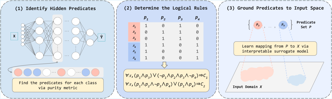
The image depicts a three-step pipeline for creating interpretable machine learning models. The pipeline aims to identify hidden predicates within a neural network, determine logical rules based on these predicates, and then ground these predicates back into the input space. The diagram is divided into three distinct sections, each representing a step in the process.
### Components/Axes
The diagram consists of three main sections, labeled (1), (2), and (3). Each section contains a visual representation of the step, along with accompanying text.
* **(1) Identify Hidden Predicates:** Shows a neural network with input 'X' and output 'Y'. Below the network is a row of colored circles representing classes, with the text "Find the predicates for each class via purity metric".
* **(2) Determine the Logical Rules:** Presents a truth table with rows labeled x1 to x6 and columns labeled P1 to P4. Below the table is a set of logical rules expressed in predicate logic.
* **(3) Ground Predicates to Input Space:** Shows a set of predicates (P1, P2, P3) and a mapping from the predicate space to the input space 'X' using an interpretable surrogate model. Below is a representation of the input domain 'X'.
### Detailed Analysis or Content Details
**Section (1): Identify Hidden Predicates**
* The neural network has an input layer labeled 'X', several hidden layers (approximately 4), and an output layer labeled 'Y'.
* The connections between layers are represented by lines with circular nodes.
* Below the network are six colored circles, alternating between two colors (approximately light blue and light orange). These represent the classes identified by the purity metric.
**Section (2): Determine the Logical Rules**
* The truth table has 6 rows (x1 to x6) and 4 columns (P1 to P4).
* The table contains binary values (0 and 1).
* x1: 1, 0, 1, 1
* x2: 0, 1, 1, 0
* x3: 1, 1, 0, 1
* x4: 1, 1, 0, 1
* x5: 1, 0, 0, 1
* x6: 0, 1, 0, 1
* The logical rules are:
* ∀x1 (P1 ∧ P3) ∨ (¬P1 ∧ P2 ∧ ¬P3) = C1
* ∀x1 (P1 ∧ ¬P2 ∧ ¬P3) ∨ (¬P1 ∧ P2) = C2
**Section (3): Ground Predicates to Input Space**
* The predicate set 'P' consists of P1, P2, and P3.
* The text states "Learn mapping from P to X via interpretable surrogate model".
* The input domain 'X' is represented as a distorted rectangle.
### Key Observations
* The pipeline progresses from a complex neural network to a set of interpretable logical rules.
* The truth table in section (2) provides a discrete representation of the relationships between predicates and input variables.
* Section (3) highlights the importance of grounding the abstract predicates back into the original input space for practical interpretation.
* The use of a "purity metric" suggests a method for identifying the most relevant predicates for each class.
### Interpretation
This diagram illustrates a method for making "black box" machine learning models, specifically neural networks, more interpretable. The process involves extracting hidden predicates (features) from the network, representing these predicates as logical rules, and then mapping these rules back to the original input space. This allows humans to understand *why* the model is making certain predictions.
The truth table in section (2) is crucial, as it defines the logical relationships between the predicates (P1-P4) and the input variables (x1-x6). The logical rules derived from this table provide a concise and human-readable explanation of the model's decision-making process.
The final step, grounding the predicates to the input space, is essential for translating the abstract rules into concrete insights about the data. The use of an "interpretable surrogate model" suggests that a simpler, more transparent model is used to approximate the mapping from predicates to inputs, further enhancing interpretability.
The alternating colors of the circles in section (1) suggest a binary classification problem, where the model is distinguishing between two classes. The pipeline aims to uncover the underlying logic that the model uses to make these classifications. The diagram suggests a focus on rule-based explanations, which are often preferred for their transparency and ease of understanding.