## Technical Document: Symbolic Regression for Periodic Hill Turbulence Modeling
### Overview
This document outlines the task of symbolic regression for modeling periodic hill turbulence. It details the flow case context, evaluation rule, tensor bases used, and the assembly of predicted anisotropy.
### Components/Axes
The document is structured into several sections:
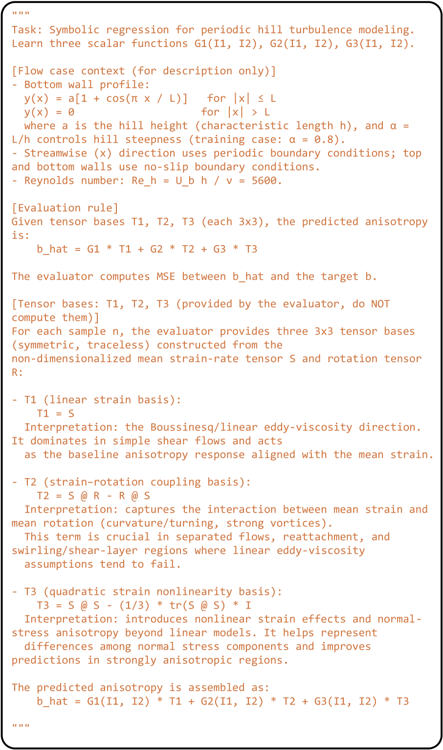
1. **Task Definition:** Describes the objective of learning three scalar functions G1, G2, and G3, which depend on invariants I1 and I2.
2. **Flow Case Context:** Defines the bottom wall profile using equations and parameters like hill height (a), characteristic length (h), and a steepness control parameter (alpha). It also specifies boundary conditions and the Reynolds number.
3. **Evaluation Rule:** Explains how the predicted anisotropy (b_hat) is calculated using tensor bases T1, T2, and T3, along with the scalar functions G1, G2, and G3. It also mentions the use of Mean Squared Error (MSE) for evaluation.
4. **Tensor Bases:** Describes the three tensor bases (T1, T2, T3) and their interpretations:
* T1 (linear strain basis): Represents the Boussinesq/linear eddy-viscosity direction.
* T2 (strain-rotation coupling basis): Captures the interaction between mean strain and mean rotation.
* T3 (quadratic strain nonlinearity basis): Introduces nonlinear strain effects and normal-stress anisotropy.
5. **Predicted Anisotropy Assembly:** Shows how the predicted anisotropy (b_hat) is assembled using the scalar functions and tensor bases.
### Detailed Analysis or ### Content Details
**Task Definition:**
* Objective: Learn three scalar functions: G1(I1, I2), G2(I1, I2), G3(I1, I2).
**Flow Case Context:**
* Bottom Wall Profile:
* y(x) = a[1 + cos(πx / L)] for |x| ≤ L
* y(x) = 0 for |x| > L
* 'a' is the hill height (characteristic length h).
* α = L/h controls hill steepness (training case: α = 0.8).
* Streamwise (x) direction: Periodic boundary conditions.
* Top and bottom walls: No-slip boundary conditions.
* Reynolds number: Re_h = U_b h / v = 5600.
**Evaluation Rule:**
* Given tensor bases T1, T2, T3 (each 3x3), the predicted anisotropy is:
* b_hat = G1 \* T1 + G2 \* T2 + G3 \* T3
* The evaluator computes MSE between b_hat and the target b.
**Tensor Bases:**
* Tensor bases T1, T2, T3 (provided by the evaluator, do NOT compute them).
* For each sample n, the evaluator provides three 3x3 tensor bases (symmetric, traceless) constructed from the non-dimensionalized mean strain-rate tensor S and rotation tensor R.
* **T1 (linear strain basis):**
* T1 = S
* Interpretation: Boussinesq/linear eddy-viscosity direction. Dominates in simple shear flows and acts as the baseline anisotropy response aligned with the mean strain.
* **T2 (strain-rotation coupling basis):**
* T2 = S @ R - R @ S
* Interpretation: Captures the interaction between mean strain and mean rotation (curvature/turning, strong vortices). Crucial in separated flows, reattachment, and swirling/shear-layer regions where linear eddy-viscosity assumptions tend to fail.
* **T3 (quadratic strain nonlinearity basis):**
* T3 = S @ S - (1/3) \* tr(S @ S) \* I
* Interpretation: Introduces nonlinear strain effects and normal-stress anisotropy beyond linear models. Helps represent differences among normal stress components and improves predictions in strongly anisotropic regions.
**Predicted Anisotropy Assembly:**
* b_hat = G1(I1, I2) \* T1 + G2(I1, I2) \* T2 + G3(I1, I2) \* T3
### Key Observations
* The document provides a structured approach to modeling turbulence over a periodic hill.
* It uses symbolic regression to learn scalar functions that relate to tensor bases.
* The tensor bases represent different aspects of the flow, including linear strain, strain-rotation coupling, and quadratic strain nonlinearity.
* The predicted anisotropy is assembled as a linear combination of these tensor bases, weighted by the learned scalar functions.
### Interpretation
The document describes a methodology for modeling complex turbulent flows, specifically over a periodic hill. The approach uses symbolic regression to learn relationships between flow invariants and tensor bases that represent different physical phenomena. By combining these elements, the model aims to predict the anisotropy of the turbulence, which is crucial for understanding and simulating such flows. The use of different tensor bases allows the model to capture various aspects of the flow, including linear and nonlinear effects, as well as the interaction between strain and rotation. The ultimate goal is to improve the accuracy of turbulence models in complex flow scenarios where traditional linear eddy-viscosity assumptions may not be valid.