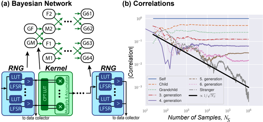
## [Technical Diagram and Chart]: Bayesian Network and Correlation Analysis ### Overview The image is a composite figure containing two distinct but related technical illustrations. Panel (a) is a schematic diagram of a **Bayesian Network** coupled with a hardware implementation block diagram. Panel (b) is a **log-log line chart** titled "Correlations," plotting the absolute value of correlation against the number of samples for various generational relationships. The overall figure appears to describe a system for generating correlated random variables and analyzing how their statistical correlation decays with sample size and generational distance. ### Components/Axes #### **Panel (a): Bayesian Network** * **Structure:** A directed acyclic graph (DAG) showing probabilistic dependencies. * **Nodes (Top Section):** * **Root Nodes:** `GF` (Grandfather), `GM` (Grandmother). * **First Generation:** `F2`, `M2`, `F1`, `M1` (likely representing Fathers and Mothers). * **Second Generation (Grandchildren):** `G61`, `G62`, `G63`, `G64`. Ellipses (`...`) indicate additional nodes in the sequence. * **Arrows:** Green arrows indicate the direction of probabilistic influence or data flow from parents to children. * **Hardware Implementation (Bottom Section):** * **Left RNG Block:** A blue box labeled `RNG` containing two sub-blocks, each with a `LUT` (Look-Up Table) and an `LFSR` (Linear Feedback Shift Register). An arrow points from this block to the Bayesian Network nodes. * **Kernel Block:** A green box labeled `Kernel` containing a `GFT LUT` and a `Multiply & Accumulate` unit. It receives input from the left RNG. * **Right RNG Block:** Another blue `RNG` block, identical in structure to the left one, receiving input from the Kernel. * **Data Flow:** Arrows show data flowing from the left RNG to the Kernel, then to the right RNG. Both RNG blocks have outputs labeled "to data collector." #### **Panel (b): Correlations Chart** * **Chart Type:** Line chart on a log-log scale. * **X-Axis:** * **Label:** `Number of Samples, N_S` * **Scale:** Logarithmic, ranging from `10^1` to `10^6`. * **Y-Axis:** * **Label:** `|Correlation|` * **Scale:** Logarithmic, ranging from `10^-3` to `10^0` (i.e., 0.001 to 1). * **Legend (Bottom-Left Corner):** Contains 9 entries, each with a specific line style and color: 1. `Self` - Solid blue line. 2. `Child` - Dashed orange line. 3. `Grandchild` - Dotted green line. 4. `3. generation` - Dash-dot red line. 5. `4. generation` - Solid purple line. 6. `5. generation` - Dashed brown line. 7. `6. generation` - Dotted pink line. 8. `Stranger` - Dash-dot gray line. 9. `∝ 1/√N_S` - Solid black line (theoretical reference). ### Detailed Analysis #### **Panel (a) Analysis** The diagram illustrates a generative model where random number generators (RNGs) feed into a processing kernel to produce samples for a Bayesian Network. The network models familial relationships across three generations (Grandparents -> Parents -> Grandchildren). The hardware blocks (RNG, Kernel) suggest a method for efficiently generating correlated random variables that adhere to the network's structure. #### **Panel (b) Analysis - Data Series Trends** * **`Self` (Blue):** Remains nearly constant at a very high correlation (~0.9-1.0) across all sample sizes. This is the baseline, representing perfect correlation of a variable with itself. * **`Child` (Orange):** Starts high (~0.5 at N_S=10^1), shows a slight initial dip, then stabilizes around 0.4-0.5 for N_S > 10^2. * **`Grandchild` (Green):** Follows a similar pattern to `Child` but at a lower level, stabilizing around 0.2-0.3. * **`3. generation` (Red):** Starts around 0.3, decays more noticeably than `Child`/`Grandchild`, and stabilizes near 0.1 for large N_S. * **`4. generation` (Purple):** Shows significant initial volatility (dips below 0.01 at N_S~10^2) before recovering and stabilizing around 0.05-0.08. * **`5. generation` (Brown) & `6. generation` (Pink):** Both show a general downward trend with noise. `5th gen` stabilizes near 0.02-0.03, while `6th gen` is lower, near 0.01-0.02. * **`Stranger` (Gray):** Exhibits the strongest decay. It starts near 0.1 but plummets with high variance, falling below 0.001 by N_S=10^6. Its trend most closely follows the theoretical black line. * **Theoretical Line (`∝ 1/√N_S`, Black):** A straight line on the log-log plot with a slope of -0.5, representing the expected decay of correlation for independent samples as sample size increases. ### Key Observations 1. **Hierarchy of Correlation:** There is a clear, ordered hierarchy: `Self` > `Child` > `Grandchild` > `3rd gen` > `4th gen` > `5th gen` > `6th gen` > `Stranger`. Correlation decreases with increasing generational distance. 2. **Asymptotic Behavior:** Most series (except `Stranger` and the theoretical line) appear to reach a non-zero asymptotic correlation floor for large N_S (>10^4). This suggests persistent, inherent correlation in the generated variables beyond random chance. 3. **`Stranger` vs. Theory:** The `Stranger` correlation decays roughly in line with the `1/√N_S` law, indicating that unrelated variables in this system behave like independent random samples in the long run. 4. **Volatility at Low N_S:** Several series, particularly `4th generation` and `Stranger`, show high volatility and deep dips at low sample counts (10^1 to 10^3), which smooth out as N_S increases. ### Interpretation This figure demonstrates a method for generating correlated random variables within a defined Bayesian network structure and quantifies the persistence of those correlations. * **System Purpose:** The hardware diagram (a) proposes an efficient RNG-Kernel-RNG pipeline to generate data that conforms to the probabilistic dependencies of the familial Bayesian network. The "data collector" outputs are the samples used for the analysis in (b). * **Meaning of Correlations:** The chart (b) answers: "How well does the generated data preserve the intended familial relationships as we collect more samples?" The high, stable correlations for close relations (`Child`, `Grandchild`) confirm the system successfully embeds these dependencies. The decaying correlations for distant relations show the influence weakens over generations. * **The `Stranger` Baseline:** The `Stranger` line is crucial. It acts as a control, showing the correlation expected between variables with no intended relationship in the network. Its adherence to the `1/√N_S` law validates that the system's noise behaves predictably. * **Persistent Correlation Floor:** The fact that most familial correlations do not decay to zero (unlike `Stranger`) is the key finding. It indicates the generative process creates a **persistent statistical dependency** that is not washed out by large sample sizes. This could be desirable for simulations where familial or network-based correlations must be maintained, or an artifact to be aware of in statistical testing. * **Peircean Investigation:** From a semiotic perspective, the `1/√N_S` line is an **icon** of statistical independence. The familial correlation lines are **indices** pointing to the underlying causal structure (the Bayesian network). The hardware diagram is the **symbol** explaining the mechanism that creates those indexed relationships. The chart proves the symbol's implementation successfully generates the indexed effects.