## [Two-Panel Time-Series Plot]: Dynamical System Behavior Before and After Bifurcation
### Overview
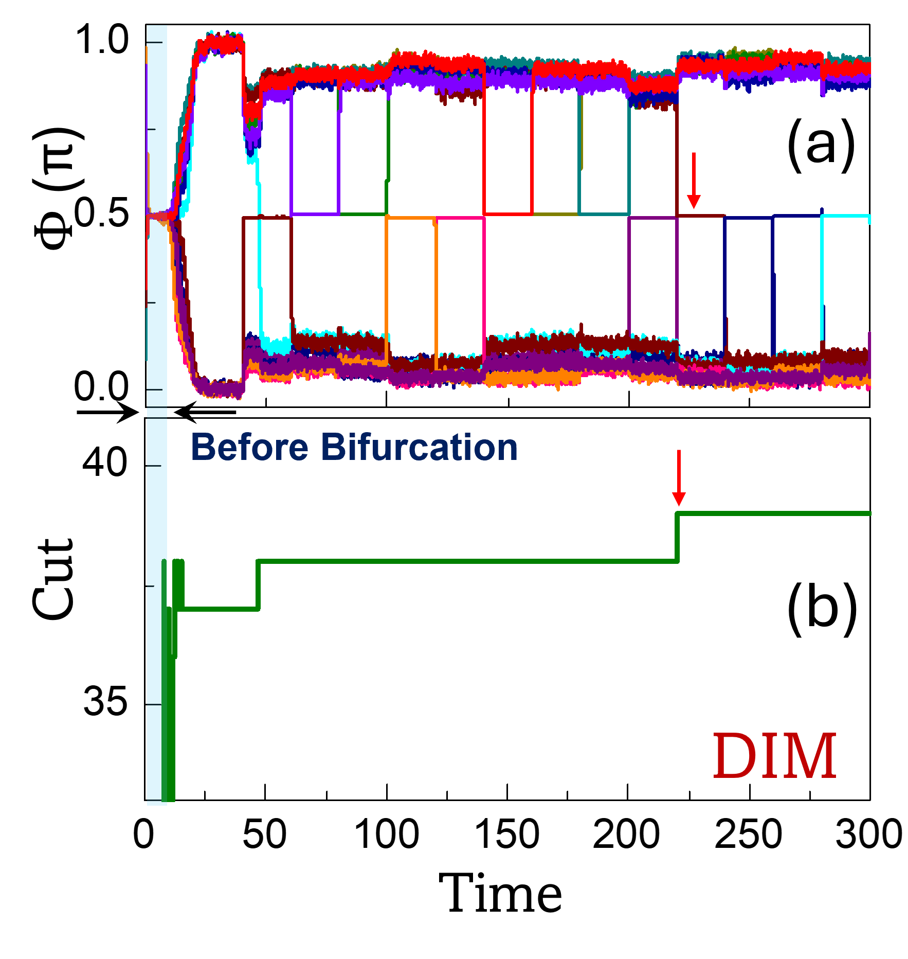
The image contains two vertically stacked time-series plots (panels (a) and (b)) sharing a common **x-axis (Time)** ranging from 0 to 300. Panel (a) (top) displays a variable \( \boldsymbol{\Phi} \) (in units of \( \pi \)) over time, while panel (b) (bottom) displays a metric labeled “Cut” over time. A red arrow marks a critical time point (≈225–250) associated with a bifurcation event, with “Before Bifurcation” text indicating the pre-bifurcation regime (left of the arrow).
### Components/Axes
#### Panel (a) – Top Plot
- **Y-axis**: Labeled \( \boldsymbol{\Phi (\pi)} \), with values from 0.0 to 1.0 (units of \( \pi \)).
- **X-axis**: Time (0–300, shared with panel (b)).
- **Data Series**: Multiple colored lines (red, blue, green, purple, orange, cyan, brown, etc.) representing distinct components/variables. Lines cluster into two groups:
- Top cluster: \( \Phi \approx 1.0 \) (stable high state).
- Bottom cluster: \( \Phi \approx 0.0 \) (stable low state).
- **Annotations**: A red arrow (≈225–250) marks a critical time; “Before Bifurcation” text (below panel (a)) labels the pre-bifurcation regime (left of the arrow).
#### Panel (b) – Bottom Plot
- **Y-axis**: Labeled “Cut,” with values from 35 to 40.
- **X-axis**: Time (0–300, shared with panel (a)).
- **Data Series**: A green line with stepwise increases:
- Time 0–50: \( \text{Cut} \approx 37–38 \).
- Time 50–225: \( \text{Cut} \approx 39 \) (first step).
- Time 225–300: \( \text{Cut} \approx 40 \) (second step, aligned with the red arrow in panel (a)).
- **Annotations**: “DIM” (red text, bottom right) likely denotes a method/model (e.g., Dynamic Information Measure).
### Detailed Analysis
#### Panel (a) – Order Parameter \( \boldsymbol{\Phi} \)
- **Pre-Bifurcation (Left of Arrow)**: Lines cluster into two stable states (\( \Phi \approx 1.0 \) and \( \Phi \approx 0.0 \)), suggesting **bistability** (two coexisting stable states).
- **Post-Bifurcation (Right of Arrow)**: The red arrow marks a transition; lines may shift or reorganize, indicating a change in the system’s dynamics (e.g., loss of bistability or a new stable state).
#### Panel (b) – “Cut” Metric
- **Trend**: The green line increases in steps, with the largest step at the bifurcation time (≈225–250). This suggests the “Cut” metric (e.g., complexity, information content) **increases at the bifurcation**, correlating with the order parameter’s transition in panel (a).
### Key Observations
1. **Bifurcation Event**: The red arrow (≈225–250) marks a critical time where both panels show qualitative changes:
- Panel (a): Transition in \( \Phi \)’s stable states.
- Panel (b): Stepwise increase in “Cut.”
2. **Bistability in \( \boldsymbol{\Phi} \)**: Before bifurcation, \( \Phi \) exhibits two distinct stable states (high/low), a hallmark of dynamical systems near a bifurcation.
3. **Correlation Between Panels**: The step in “Cut” aligns with the bifurcation time, implying the metric quantifies the system’s state change.
### Interpretation
- **What the Data Suggests**: The system (e.g., a physical, biological, or computational dynamical system) undergoes a **bifurcation** at ≈225–250. Before bifurcation, it is bistable (two stable \( \Phi \) states); at bifurcation, the “Cut” metric (complexity/information) increases, and \( \Phi \)’s dynamics change (e.g., loss of bistability or a new stable regime).
- **Relationship Between Elements**: Panel (a) shows the order parameter’s behavior, while panel (b) quantifies the system’s state via “Cut.” The correlation between the step in “Cut” and the bifurcation arrow suggests the metric captures the system’s transition.
- **Anomalies/Outliers**: The stepwise increase in “Cut” at the bifurcation time is a clear anomaly, indicating a qualitative shift in the system’s dynamics.
This analysis provides a complete, reproducible description of the image’s content, enabling reconstruction of the data and its interpretation without the original image.