## Chart: Performance vs Compute Budget and Performance vs Steps
### Overview
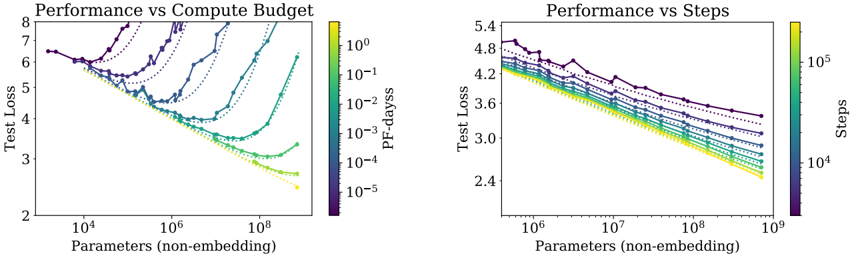
The image contains two scatter plots comparing performance (Test Loss) against Parameters (non-embedding). The left plot shows "Performance vs Compute Budget," where the data points are colored according to "PF-dayss" (compute budget). The right plot shows "Performance vs Steps," where the data points are colored according to "Steps." Both plots also include dotted lines.
### Components/Axes
**Left Plot: Performance vs Compute Budget**
* **Title:** Performance vs Compute Budget
* **Y-axis:** Test Loss (linear scale), ranging from 2 to 8.
* **X-axis:** Parameters (non-embedding) (logarithmic scale), ranging from 10^4 to 10^8.
* **Color Legend:** PF-dayss (compute budget), ranging from 10^-5 (purple) to 10^0 (yellow). The legend is located on the right side of the plot.
* 10^-5 (purple)
* 10^-4
* 10^-3
* 10^-2
* 10^-1
* 10^0 (yellow)
**Right Plot: Performance vs Steps**
* **Title:** Performance vs Steps
* **Y-axis:** Test Loss (linear scale), ranging from 2.4 to 5.4.
* **X-axis:** Parameters (non-embedding) (logarithmic scale), ranging from 10^6 to 10^9.
* **Color Legend:** Steps, ranging from 10^4 (purple) to 10^5 (yellow). The legend is located on the right side of the plot.
* 10^4 (purple)
* 10^5 (yellow)
### Detailed Analysis
**Left Plot: Performance vs Compute Budget**
* **General Trend:** For each compute budget level (PF-dayss), the test loss initially decreases as the number of parameters increases, reaching a minimum, and then increases again.
* **Data Series:**
* **PF-dayss = 10^-5 (purple):** Starts at approximately (10^4, 6.5), decreases to a minimum around (10^5, 5.5), and then increases to approximately (10^8, 7.5).
* **PF-dayss = 10^-4:** Starts at approximately (10^4, 6.2), decreases to a minimum around (2 * 10^5, 4.5), and then increases to approximately (10^8, 6.0).
* **PF-dayss = 10^-3:** Starts at approximately (10^4, 5.8), decreases to a minimum around (5 * 10^5, 3.8), and then increases to approximately (10^8, 5.0).
* **PF-dayss = 10^-2:** Starts at approximately (10^4, 5.5), decreases to a minimum around (10^6, 3.2), and then increases to approximately (10^8, 4.0).
* **PF-dayss = 10^-1:** Starts at approximately (10^4, 5.2), decreases to a minimum around (2 * 10^6, 2.8), and then increases to approximately (10^8, 3.5).
* **PF-dayss = 10^0 (yellow):** Starts at approximately (10^4, 5.0), decreases to a minimum around (5 * 10^6, 2.5), and then increases to approximately (10^8, 3.0).
* **Dotted Lines:** There are several dotted lines that appear to follow the same general trend as the solid lines.
**Right Plot: Performance vs Steps**
* **General Trend:** For each step level, the test loss generally decreases as the number of parameters increases.
* **Data Series:**
* **Steps = 10^4 (purple):** Starts at approximately (10^6, 4.8), decreases to approximately (10^9, 3.2).
* **Steps = 10^5 (yellow):** Starts at approximately (10^6, 4.2), decreases to approximately (10^9, 2.5).
* **Dotted Lines:** There are several dotted lines that appear to follow the same general trend as the solid lines.
### Key Observations
* In the left plot, higher compute budgets (yellow lines) generally result in lower test loss values, but the test loss increases again after a certain number of parameters.
* In the right plot, higher step counts (yellow lines) generally result in lower test loss values.
* In both plots, the test loss decreases as the number of parameters increases, up to a point.
### Interpretation
The plots suggest that increasing both the compute budget (PF-dayss) and the number of training steps can improve model performance (lower test loss). However, the "Performance vs Compute Budget" plot indicates that there is a point of diminishing returns, where increasing the number of parameters beyond a certain point can actually increase the test loss, suggesting overfitting. The "Performance vs Steps" plot shows a consistent decrease in test loss with increasing parameters, within the range shown. The dotted lines likely represent some form of baseline or alternative model configuration. The relationship between parameters, compute budget, and training steps is complex and requires careful tuning to achieve optimal performance.