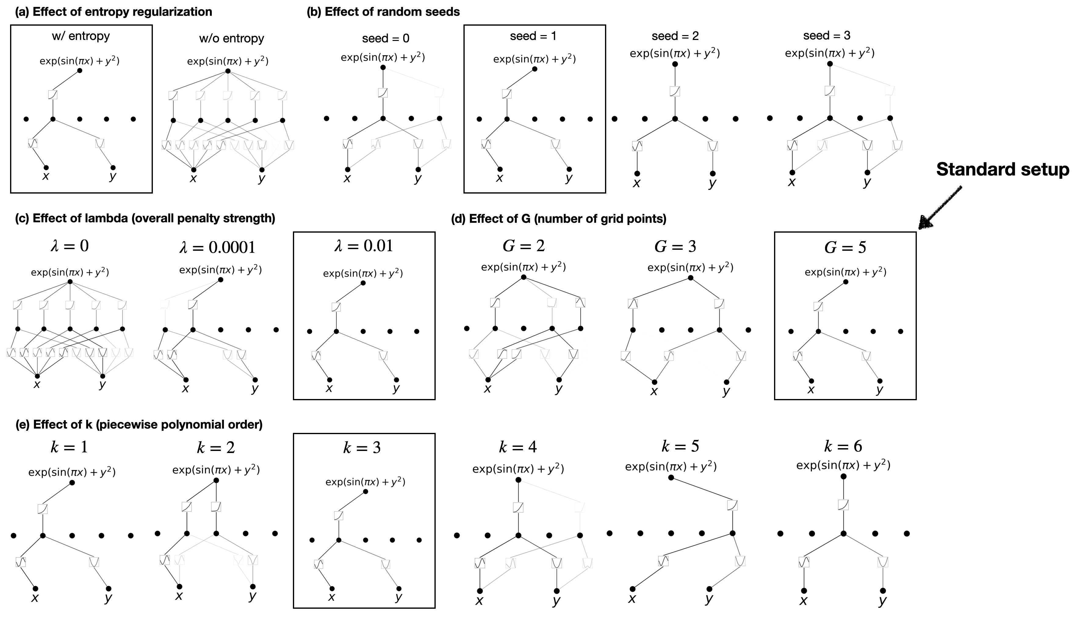
# Technical Document Extraction: Network Structure Analysis Diagram ## Diagram Overview The image presents a comparative analysis of network structures under varying parameters, organized into five panels (a)-(e). Each panel demonstrates how specific variables influence node connections and network topology. --- ### Panel (a): Effect of Entropy Regularization **Title**: Effect of entropy regularization **Sub-labels**: - Left box: `w/ entropy` - Equation: `exp(sin(πx) + y²)` - Diagram: Sparse connections between nodes `x` and `y` - Right box: `w/o entropy` - Equation: `exp(sin(πx) + y²)` - Diagram: Dense interconnections between nodes **Key Observations**: - Entropy regularization reduces network connectivity density. - Node labels: `x` (input), `y` (output). --- ### Panel (b): Effect of Random Seeds **Title**: Effect of random seeds **Sub-labels**: - `seed = 0` - Equation: `exp(sin(πx) + y²)` - Diagram: Moderate connectivity - `seed = 1` - Equation: `exp(sin(πx) + y²)` - Diagram: Increased branching - `seed = 2` - Equation: `exp(sin(πx) + y²)` - Diagram: Complex inter-node paths - `seed = 3` - Equation: `exp(sin(πx) + y²)` - Diagram: Highly optimized topology **Key Observations**: - Random seeds introduce variability in network architecture. - All configurations share the same base equation but differ in structural outcomes. --- ### Panel (c): Effect of Lambda (Overall Penalty Strength) **Title**: Effect of lambda (overall penalty strength) **Sub-labels**: - `λ = 0` - Equation: `exp(sin(πx) + y²)` - Diagram: Fully connected network - `λ = 0.0001` - Equation: `exp(sin(πx) + y²)` - Diagram: Slight reduction in connections - `λ = 0.01` - Equation: `exp(sin(πx) + y²)` - Diagram: Significant sparsity **Key Observations**: - Higher λ values enforce stricter penalties, reducing network density. - Node labels remain consistent (`x`, `y`). --- ### Panel (d): Effect of G (Number of Grid Points) **Title**: Effect of G (number of grid points) **Sub-labels**: - `G = 2` - Equation: `exp(sin(πx) + y²)` - Diagram: Minimal grid-based connections - `G = 3` - Equation: `exp(sin(πx) + y²)` - Diagram: Intermediate grid complexity - `G = 5` (Standard setup) - Equation: `exp(sin(πx) + y²)` - Diagram: Balanced grid structure **Key Observations**: - `G = 5` is marked as the "Standard setup" with optimal grid resolution. - Increasing G enhances spatial resolution in the network. --- ### Panel (e): Effect of k (Piecewise Polynomial Order) **Title**: Effect of k (piecewise polynomial order) **Sub-labels**: - `k = 1` - Equation: `exp(sin(πx) + y²)` - Diagram: Linear node relationships - `k = 2` - Equation: `exp(sin(πx) + y²)` - Diagram: Quadratic interactions - `k = 3` - Equation: `exp(sin(πx) + y²)` - Diagram: Cubic complexity - `k = 4` - Equation: `exp(sin(πx) + y²)` - Diagram: Higher-order polynomial paths - `k = 5` - Equation: `exp(sin(πx) + y²)` - Diagram: Advanced polynomial modeling - `k = 6` - Equation: `exp(sin(πx) + y²)` - Diagram: Maximum polynomial flexibility **Key Observations**: - Higher k values enable more complex node interactions. - All configurations use the same base equation but vary in functional approximation depth. --- ### Cross-Referenced Elements - **Equations**: All panels use `exp(sin(πx) + y²)` as the base function, with structural differences arising from parameter adjustments. - **Node Labels**: Consistent use of `x` (input) and `y` (output) across all diagrams. - **Standard Setup**: Explicitly marked in panel (d) for `G = 5`. --- ### Summary This diagram systematically explores how entropy regularization, random seeds, penalty strength (λ), grid resolution (G), and polynomial order (k) influence network topology. Each parameter adjustment alters connectivity patterns while maintaining the core mathematical formulation. The "Standard setup" (`G = 5`) serves as a reference point for optimal grid-based performance.