## Diagram: Sparse vs. Non-Sparse Neural Networks for Addition
### Overview
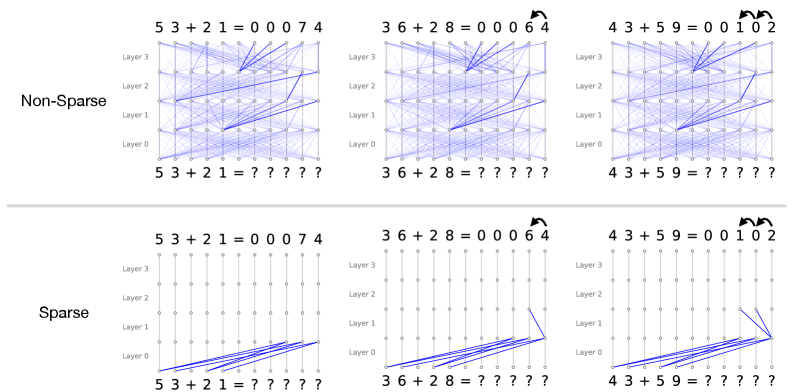
The image presents a comparative diagram illustrating the difference between non-sparse and sparse neural networks in the context of performing addition. It shows how connections between layers are structured in both types of networks for three different addition problems: 5+3+2+1, 3+6+2+8, and 4+3+5+9. The diagram highlights the reduced connectivity in sparse networks compared to non-sparse networks.
### Components/Axes
* **Title:** The image is implicitly titled by the labels "Non-Sparse" and "Sparse".
* **Layers:** Each network diagram has four layers labeled "Layer 0", "Layer 1", "Layer 2", and "Layer 3".
* **Nodes:** Each layer consists of 10 nodes, represented by small circles.
* **Connections:** Blue lines represent connections between nodes in adjacent layers.
* **Input:** Each network takes four single-digit numbers as input (e.g., 5, 3, 2, 1). These are presented as an addition problem at the bottom of each network diagram (e.g., "5+3+2+1=?????").
* **Output:** The output of each network is a five-digit number, representing the sum of the input digits. This is shown at the top of each network diagram (e.g., "5+3+2+1=00074").
* **Arrows:** Curved arrows above the output indicate the direction of carry-over operations.
### Detailed Analysis
**Top Row: Non-Sparse Networks**
* **General Structure:** In the non-sparse networks, each node in a layer is connected to every node in the adjacent layers. This creates a dense network of connections.
* **Addition Problem 1: 5+3+2+1=00074**
* Input: 5, 3, 2, 1
* Output: 00074
* **Addition Problem 2: 3+6+2+8=00064**
* Input: 3, 6, 2, 8
* Output: 00064
* Carry-over: A single curved arrow indicates a carry-over operation.
* **Addition Problem 3: 4+3+5+9=00102**
* Input: 4, 3, 5, 9
* Output: 00102
* Carry-over: Two curved arrows indicate two carry-over operations.
**Bottom Row: Sparse Networks**
* **General Structure:** In the sparse networks, each node in a layer is connected to only a few nodes in the adjacent layers. This creates a sparse network of connections.
* **Addition Problem 1: 5+3+2+1=00074**
* Input: 5, 3, 2, 1
* Output: 00074
* Connections: The input nodes (5, 3, 2, 1) in Layer 0 are connected to a limited number of nodes in Layer 1.
* **Addition Problem 2: 3+6+2+8=00064**
* Input: 3, 6, 2, 8
* Output: 00064
* Carry-over: A single curved arrow indicates a carry-over operation.
* Connections: The input nodes (3, 6, 2, 8) in Layer 0 are connected to a limited number of nodes in Layer 1.
* **Addition Problem 3: 4+3+5+9=00102**
* Input: 4, 3, 5, 9
* Output: 00102
* Carry-over: Two curved arrows indicate two carry-over operations.
* Connections: The input nodes (4, 3, 5, 9) in Layer 0 are connected to a limited number of nodes in Layer 1.
### Key Observations
* **Connectivity:** The primary difference between the two types of networks is the density of connections. Non-sparse networks have full connectivity, while sparse networks have limited connectivity.
* **Complexity:** Non-sparse networks are more complex due to the higher number of connections.
* **Efficiency:** Sparse networks are potentially more efficient in terms of computation and memory usage due to the reduced number of connections.
* **Carry-over Operations:** The curved arrows indicate carry-over operations, which are essential for accurate addition.
### Interpretation
The diagram illustrates the concept of sparsity in neural networks and its potential benefits. Sparse networks can achieve similar results to non-sparse networks with fewer connections, which can lead to improved efficiency and reduced computational cost. The specific example of addition highlights how sparsity can be applied to a simple arithmetic task. The carry-over arrows indicate the complexity of even simple addition when implemented in a neural network architecture. The diagram suggests that sparse networks can be a viable alternative to dense networks in certain applications, particularly where computational resources are limited.