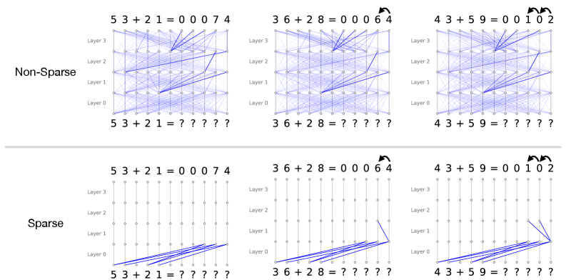
## Diagram: Neural Network Attention Patterns: Non-Sparse vs. Sparse in Addition Tasks ### Overview This image presents a comparative visualization of internal information flow (likely attention weights or activation pathways) within a multi-layer neural network performing multi-digit addition. It contrasts two architectural or regularization approaches: "Non-Sparse" (top row) and "Sparse" (bottom row). The comparison is demonstrated across three distinct addition problems of increasing algorithmic complexity: no carry-over, a single carry-over, and a double carry-over. The primary language present in the image is English (labels such as "Non-Sparse", "Sparse", "Layer"). The rest of the text consists of mathematical equations and symbols. ### Components/Axes **Global Layout:** * **Rows:** Two main horizontal sections separated by a light gray line. * Top Row: Labeled **"Non-Sparse"** on the far left. * Bottom Row: Labeled **"Sparse"** on the far left. * **Columns:** Three vertical columns representing different addition problems. * Left Column: $53 + 21$ (No carry) * Middle Column: $36 + 28$ (Single carry) * Right Column: $43 + 59$ (Double carry) **Individual Diagram Structure (Applies to all 6 sub-diagrams):** * **Y-Axis (Vertical):** Represents the depth of the neural network, labeled on the left side of each diagram from bottom to top: * `Layer 0` * `Layer 1` * `Layer 2` * `Layer 3` * **X-Axis Bottom (Input Sequence):** The sequence of tokens fed into the model. * Format: `[Digit] [Digit] + [Digit] [Digit] = ? ? ? ? ?` * **X-Axis Top (Output Sequence):** The sequence of tokens produced by the model. * Format: `[Digit] [Digit] + [Digit] [Digit] = [Pad] [Pad] [Pad] [Digit] [Digit]` (Note: leading zeros are used as padding). * **Nodes:** Small circles arranged in a grid (11 columns wide by 4 layers high). Each node represents a token's representation at a specific layer. * **Edges (Lines):** Blue lines connecting nodes between adjacent layers. These represent the flow of information or attention weights. Thicker/darker lines indicate stronger connections. * **Annotations:** Curved black arrows above the output sequences in the middle and right columns, indicating mathematical "carry" operations. --- ### Detailed Analysis & Content Details #### Section 1: Non-Sparse Model (Top Row) *Visual Trend:* Across all three problems, the Non-Sparse model exhibits a highly entangled, dense web of connections. Information from almost every node in a lower layer is broadcast to multiple nodes in the subsequent layer. * **Left Diagram (No Carry):** * **Input:** `5 3 + 2 1 = ? ? ? ? ?` * **Output:** `5 3 + 2 1 = 0 0 0 7 4` * **Flow:** A dense mesh of blue lines connects Layer 0 through Layer 3. While dense, thicker blue lines can be seen routing information from the input digits (`5, 3, 2, 1`) diagonally towards the right side of the network, specifically targeting the nodes that will output `7` and `4`. * **Middle Diagram (Single Carry):** * **Input:** `3 6 + 2 8 = ? ? ? ? ?` * **Output:** `3 6 + 2 8 = 0 0 0 6 4` * **Annotation:** A curved black arrow points from the `4` to the `6` in the output, denoting the carry from $6+8=14$. * **Flow:** Similar dense mesh. Stronger attention pathways are visible converging on the nodes responsible for outputting `6` and `4`. The network is solving the carry, but the mechanism is distributed across many nodes and layers. * **Right Diagram (Double Carry):** * **Input:** `4 3 + 5 9 = ? ? ? ? ?` * **Output:** `4 3 + 5 9 = 0 0 1 0 2` * **Annotation:** Two curved black arrows. One from `2` to `0`, and another from `0` to `1`, denoting the cascading carries ($3+9=12$; $4+5+1=10$). * **Flow:** The densest web of the three. The model successfully calculates the output, but the internal routing is highly complex and visually uninterpretable regarding *how* the double carry is executed. #### Section 2: Sparse Model (Bottom Row) *Visual Trend:* The Sparse model exhibits a radically simplified, highly structured flow of information. The vast majority of connections are strictly vertical (identity or residual connections, where a token simply passes its state to the next layer). Diagonal connections (cross-token attention) are rare, deliberate, and highly localized. * **Left Diagram (No Carry):** * **Input:** `5 3 + 2 1 = ? ? ? ? ?` * **Output:** `5 3 + 2 1 = 0 0 0 7 4` * **Flow:** * **Layer 0 to Layer 1:** Diagonal blue lines route information from the input digits (`5, 3, 2, 1`) directly to the specific token positions that will become the output digits (`7` and `4`). * **Layer 1 to Layer 3:** Strictly vertical lines. No further cross-token communication is needed because no carry operation is required. The calculation is completed in the first layer transition. * **Middle Diagram (Single Carry):** * **Input:** `3 6 + 2 8 = ? ? ? ? ?` * **Output:** `3 6 + 2 8 = 0 0 0 6 4` * **Annotation:** Curved arrow from `4` to `6`. * **Flow:** * **Layer 0 to Layer 1:** Similar to the left diagram, inputs are routed to the output positions. * **Layer 1 to Layer 2:** A single, distinct diagonal blue line appears. It connects the node at the ones-place output position (under the `4`) to the node at the tens-place output position (under the `6`). This line perfectly mirrors the carry annotation above it. * **Layer 2 to Layer 3:** Strictly vertical lines. * **Right Diagram (Double Carry):** * **Input:** `4 3 + 5 9 = ? ? ? ? ?` * **Output:** `4 3 + 5 9 = 0 0 1 0 2` * **Annotation:** Two curved arrows (from `2` to `0`, and `0` to `1`). * **Flow:** * **Layer 0 to Layer 1:** Inputs are routed to the output positions. * **Layer 1 to Layer 2:** Two distinct diagonal blue lines appear. 1. One line connects the ones-place position (under `2`) to the tens-place position (under `0`). 2. A second line connects the tens-place position (under `0`) to the hundreds-place position (under `1`). * These two lines perfectly mirror the double-carry annotations at the top of the diagram. * **Layer 2 to Layer 3:** Strictly vertical lines. --- ### Key Observations 1. **Entanglement vs. Isolation:** The Non-Sparse model uses a "black box" distributed representation where every layer mixes information from all tokens. The Sparse model isolates specific algorithmic steps to specific layers. 2. **Algorithmic Layering in Sparse Model:** The Sparse model demonstrates a clear, human-readable algorithm: * *Step 1 (Layer 0 $\rightarrow$ 1):* Gather operands (route inputs to output positions). * *Step 2 (Layer 1 $\rightarrow$ 2):* Execute carry operations (route information from right to left). * *Step 3 (Layer 2 $\rightarrow$ 3):* Finalize output (pass information vertically). 3. **Visualizing the "Carry":** The most striking observation is how the Sparse model physically manifests the mathematical "carry" operation as a literal diagonal connection between adjacent token positions in Layer 1 $\rightarrow$ Layer 2. ### Interpretation This diagram serves as a powerful piece of evidence in the field of Mechanistic Interpretability within machine learning. It demonstrates that standard, dense neural networks (Non-Sparse) tend to learn tasks in a highly distributed, polysemantic way that is incredibly difficult for humans to reverse-engineer. While the dense model gets the math right, it does so using a messy web of heuristics. Conversely, by applying sparsity (likely through sparse attention mechanisms or specific regularization techniques during training), the network is forced to drop unnecessary connections. This constraint forces the model to learn a clean, discrete, and highly interpretable algorithm. The Sparse model has essentially re-invented the human method of column addition: it aligns the numbers, adds the columns, and then explicitly passes the "carry" to the next column to the left in a subsequent processing step. The image proves that under the right constraints, neural networks do not have to be black boxes; they can learn human-readable, step-by-step logical circuits.