## Diagram: Comparison of Non-Sparse and Sparse Neural Network Architectures for Arithmetic Operations
### Overview
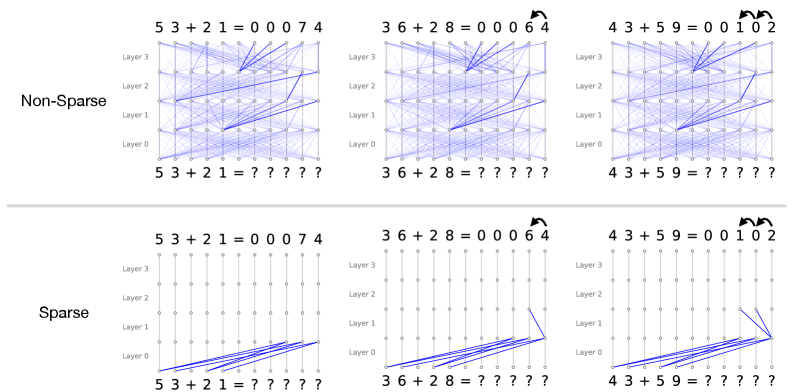
The image is a technical diagram comparing two types of neural network connectivity patterns—labeled "Non-Sparse" and "Sparse"—applied to three different addition problems. It visually demonstrates how information flows through a 4-layer network (Layer 0 to Layer 3) to compute the sum. The top half shows the "Non-Sparse" architecture with dense connections, while the bottom half shows the "Sparse" architecture with significantly fewer, targeted connections. Both architectures produce identical numerical outputs for the given problems.
### Components/Axes
* **Main Sections:** The diagram is split horizontally into two primary sections.
* **Top Section:** Labeled **"Non-Sparse"** on the left.
* **Bottom Section:** Labeled **"Sparse"** on the left.
* **Columns:** Each section contains three columns, each dedicated to a specific arithmetic problem.
* **Left Column:** Problem: `5 3 + 2 1 = ? ? ? ? ?`
* **Middle Column:** Problem: `3 6 + 2 8 = ? ? ? ? ?`
* **Right Column:** Problem: `4 3 + 5 9 = ? ? ? ? ?`
* **Network Layers (Y-Axis):** Each diagram has a vertical axis labeled with four layers, from bottom to top:
* `Layer 0`
* `Layer 1`
* `Layer 2`
* `Layer 3`
* **Nodes:** Each layer consists of a horizontal row of 11 small, grey circular nodes.
* **Connections:** Blue lines represent connections (weights) between nodes in adjacent layers.
* **Output Display:** The computed result is displayed in two places for each problem:
1. **Top of each diagram:** The full equation with the result, e.g., `5 3 + 2 1 = 0 0 0 7 4`.
2. **Bottom of each diagram:** The equation with the result represented by question marks, e.g., `5 3 + 2 1 = ? ? ? ? ?`.
* **Additional Symbols:** Small, black, curved arrow icons appear above the result in the top display for the middle and right columns in both sections.
### Detailed Analysis
**1. Non-Sparse Architecture (Top Section):**
* **Connectivity Pattern:** Extremely dense. Nearly every node in a given layer is connected to every node in the layer above it, creating a complex web of blue lines.
* **Problem 1 (53 + 21):**
* **Top Result:** `5 3 + 2 1 = 0 0 0 7 4`
* **Visual Trend:** Connections are uniformly dense across all layers (0 through 3).
* **Problem 2 (36 + 28):**
* **Top Result:** `3 6 + 2 8 = 0 0 0 6 4`
* **Visual Trend:** Dense connections, similar to Problem 1. A small black arrow icon is present above the result `6 4`.
* **Problem 3 (43 + 59):**
* **Top Result:** `4 3 + 5 9 = 0 0 1 0 2`
* **Visual Trend:** Dense connections. Two small black arrow icons are present above the result `1 0 2`.
**2. Sparse Architecture (Bottom Section):**
* **Connectivity Pattern:** Highly selective. Connections are minimal and appear to follow specific, learned pathways, primarily originating from nodes in the lower layers (Layer 0 and Layer 1).
* **Problem 1 (53 + 21):**
* **Top Result:** `5 3 + 2 1 = 0 0 0 7 4` (Identical to Non-Sparse).
* **Visual Trend:** Connections are almost exclusively from nodes in Layer 0 to nodes in Layer 1. Very few connections exist to higher layers.
* **Problem 2 (36 + 28):**
* **Top Result:** `3 6 + 2 8 = 0 0 0 6 4` (Identical to Non-Sparse).
* **Visual Trend:** Connections start in Layer 0, converge to a few nodes in Layer 1, and then a single, prominent connection path extends up to Layer 3. The black arrow icon is present.
* **Problem 3 (43 + 59):**
* **Top Result:** `4 3 + 5 9 = 0 0 1 0 2` (Identical to Non-Sparse).
* **Visual Trend:** Similar to Problem 2, with a focused pathway from lower layers to a specific node in Layer 3. Two black arrow icons are present.
### Key Observations
1. **Identical Outputs:** Despite the drastic difference in connectivity density, both the Non-Sparse and Sparse architectures compute the exact same results for all three addition problems.
2. **Connectivity Efficiency:** The Sparse architecture achieves the same result using a tiny fraction of the connections used by the Non-Sparse architecture. This suggests a model that has learned to prune irrelevant connections.
3. **Pathway Specialization:** In the Sparse diagrams, the connection patterns differ between problems (e.g., the pathway for `36+28` is distinct from `43+59`), indicating the network may develop specialized sub-circuits for different input patterns.
4. **Layer Utilization:** The Non-Sparse model uses all layers heavily. The Sparse model appears to perform significant computation in the lower layers (0 and 1), with only critical information being propagated to the highest layer (Layer 3) for the final output.
### Interpretation
This diagram is a powerful visual argument for the efficiency of **sparse neural networks** or **pruned networks**. It demonstrates that a densely connected ("Non-Sparse") network contains a vast amount of redundancy. Through training or pruning, a network can be transformed into a "Sparse" version that retains full accuracy on its task while eliminating the majority of its parameters (connections).
The **implications** are significant for computational efficiency:
* **Reduced Memory:** A sparse model requires less memory to store its weights.
* **Faster Computation:** Fewer connections mean fewer mathematical operations during the forward pass, leading to faster inference.
* **Interpretability:** The focused pathways in the sparse model are easier to analyze, potentially revealing how the network solves the arithmetic problem (e.g., which input digits contribute to which output digits).
The black arrow icons above certain results in the top display may indicate a specific operation (like a "carry" in addition) or highlight outputs that required more complex computation, which the sparse network still handles correctly with its efficient pathways. The diagram ultimately argues that intelligence (or at least, correct computation) in a neural network does not require every neuron to talk to every other neuron; it can emerge from a sparse, efficient, and structured set of connections.