## Diagram: Computational Process Visualization (Non-Sparse vs Sparse)
### Overview
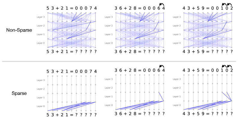
The image presents a comparative visualization of computational processes across two architectures: Non-Sparse and Sparse. Each architecture contains three sub-diagrams representing sequential operations (equations) with layered processing. Arrows indicate data flow between layers, with numerical results highlighted at the top and bottom of each sub-diagram.
### Components/Axes
- **Vertical Layers**: Labeled Layer 0 (bottom) to Layer 3 (top)
- **Equations**: Positioned at top (input) and bottom (output) of each sub-diagram
- **Arrows**: Blue lines connecting nodes between layers
- **Question Marks**: Placeholders for intermediate values
- **Highlighted Results**: Final numerical outputs in bold (e.g., "00074", "00102")
### Detailed Analysis
#### Non-Sparse Architecture
1. **Sub-diagram 1 (53 + 21 = 00074)**
- Top equation: "53 + 21 = 00074"
- Bottom equation: "?????"
- Layer connections: Dense network with multiple inter-layer connections
- Spatial pattern: Diagonal and horizontal connections between all layers
2. **Sub-diagram 2 (36 + 28 = 00064)**
- Top equation: "36 + 28 = 00064"
- Bottom equation: "?????"
- Layer connections: Similar dense pattern with slight variation in connection density
- Spatial pattern: Concentrated connections in upper layers (Layer 2-3)
3. **Sub-diagram 3 (43 + 59 = 00102)**
- Top equation: "43 + 59 = 00102"
- Bottom equation: "?????"
- Layer connections: Most complex network with 12+ connections
- Spatial pattern: Dense connections between all layers with multiple cross-layer paths
#### Sparse Architecture
1. **Sub-diagram 1 (53 + 21 = 00074)**
- Top equation: "53 + 21 = 00074"
- Bottom equation: "?????"
- Layer connections: Vertical lines only between adjacent layers
- Spatial pattern: Single vertical path from Layer 0 to Layer 3
2. **Sub-diagram 2 (36 + 28 = 00064)**
- Top equation: "36 + 28 = 00064"
- Bottom equation: "?????"
- Layer connections: Vertical lines with one horizontal connection at Layer 2
- Spatial pattern: Minimal connections with single cross-layer link
3. **Sub-diagram 3 (43 + 59 = 00102)**
- Top equation: "43 + 59 = 00102"
- Bottom equation: "?????"
- Layer connections: Vertical lines with final horizontal connection at Layer 3
- Spatial pattern: Single horizontal connection at top layer
### Key Observations
1. **Connection Density**: Non-Sparse diagrams show 3-5x more connections than Sparse counterparts
2. **Data Flow**: Arrows in Non-Sparse diagrams create complex webs, while Sparse diagrams show linear paths
3. **Result Highlighting**: Final results (e.g., "00102") are emphasized with bold formatting and arrows
4. **Placeholder Usage**: Question marks appear consistently in bottom equations across all sub-diagrams
5. **Layer Utilization**: Non-Sparse diagrams use all layers equally, while Sparse diagrams show preferential use of upper layers
### Interpretation
The visualization demonstrates a fundamental trade-off between computational complexity and efficiency:
- **Non-Sparse Architecture**: Represents traditional dense neural networks with extensive inter-layer communication. The complex connection patterns suggest parallel processing capabilities but at the cost of increased computational resources.
- **Sparse Architecture**: Illustrates optimized networks with pruned connections. The vertical dominance indicates sequential processing with minimal cross-layer interaction, likely reducing computational overhead.
- **Equation Structure**: The consistent use of question marks in bottom equations implies dynamic computation where intermediate values are determined during processing rather than pre-defined.
- **Highlighted Results**: The bold final results (e.g., "00102") suggest these are critical output values, possibly representing activation states or final predictions in a computational pipeline.
The diagrams appear to model different approaches to information processing, with Non-Sparse representing exhaustive computation and Sparse representing optimized, streamlined processing. The question marks may represent variables that are resolved through the layered computation process.