## Line Chart: Shannon and Bayesian Surprises
### Overview
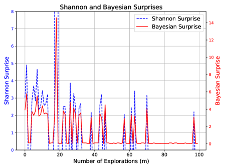
This is a dual-axis line chart comparing two metrics, "Shannon Surprise" and "Bayesian Surprise," plotted against the "Number of Explorations (m)." The chart displays how these two measures of surprise fluctuate over a sequence of 100 exploration steps.
### Components/Axes
* **Chart Title:** "Shannon and Bayesian Surprises" (centered at the top).
* **X-Axis:**
* **Label:** "Number of Explorations (m)" (centered at the bottom).
* **Scale:** Linear scale from 0 to 100, with major tick marks every 20 units (0, 20, 40, 60, 80, 100).
* **Primary Y-Axis (Left):**
* **Label:** "Shannon Surprise" (rotated vertically).
* **Scale:** Linear scale from 0 to 8, with major tick marks every 1 unit.
* **Secondary Y-Axis (Right):**
* **Label:** "Bayesian Surprise" (rotated vertically).
* **Scale:** Linear scale from 0 to 14, with major tick marks every 2 units.
* **Legend:** Located in the top-right corner of the plot area.
* **Blue Dashed Line:** "Shannon Surprise"
* **Red Solid Line:** "Bayesian Surprise"
### Detailed Analysis
**Data Series Trends:**
1. **Shannon Surprise (Blue Dashed Line):**
* **Trend:** The series is highly volatile, characterized by frequent, sharp spikes from a baseline near zero. The most prominent spike occurs at approximately m=20.
* **Key Data Points (Approximate):**
* **Highest Peak:** At m ≈ 20, Shannon Surprise reaches its maximum value of ~8.
* **Other Major Peaks:** At m ≈ 2, 8, 12, 28, 45, 62, 68, and 98, with values ranging between ~3 and ~5.
* **Baseline:** Between spikes, the value frequently returns to near 0.
2. **Bayesian Surprise (Red Solid Line):**
* **Trend:** This series also shows spiky behavior correlated with the Shannon Surprise spikes, but with a different magnitude and a slightly smoother profile in some regions. It has a notable period of very low, stable values in the latter part of the exploration sequence.
* **Key Data Points (Approximate):**
* **Highest Peak:** At m ≈ 20, Bayesian Surprise reaches its maximum value of ~14 (on the right axis).
* **Other Major Peaks:** At m ≈ 2, 8, 12, 28, 45, 62, and 98, with values ranging between ~4 and ~8.
* **Notable Low Period:** From approximately m=75 to m=95, the Bayesian Surprise remains very close to 0, with minimal fluctuation.
**Spatial & Cross-Reference Check:**
* The legend is positioned in the top-right, clearly associating the blue dashed line with Shannon Surprise and the red solid line with Bayesian Surprise.
* The major spikes in both lines are temporally aligned (e.g., at m≈20, 45, 62), confirming they are reacting to the same exploration events. The red line's peak at m≈20 is visually the tallest feature on the chart relative to its own axis.
### Key Observations
1. **Correlated Spikes:** The most significant observation is the strong temporal correlation between spikes in Shannon Surprise and Bayesian Surprise. Every major peak in one series corresponds to a peak in the other.
2. **Magnitude Difference:** The Bayesian Surprise metric reaches a higher absolute maximum (14 vs. 8) and generally has higher peak values relative to its scale compared to Shannon Surprise.
3. **Divergence in Stability:** While both metrics are volatile, the Bayesian Surprise exhibits a prolonged period of near-zero stability (m=75-95) that is not as clearly mirrored in the Shannon Surprise series, which continues to show small fluctuations.
4. **Concentration of Events:** The highest density of large surprise events occurs in the first half of the exploration sequence (m=0 to 50).
### Interpretation
This chart visualizes the information-theoretic "surprise" generated during an exploration process. The data suggests that specific exploration steps (e.g., m≈20) yielded outcomes that were highly unexpected according to both Shannon's information theory (which measures information content) and a Bayesian framework (which measures deviation from prior beliefs).
The perfect alignment of spikes indicates that events causing high Shannon information content also cause a significant update in Bayesian belief. The higher magnitude of Bayesian Surprise peaks might suggest that these events were not just informative but also strongly contradicted prior expectations. The later period of low Bayesian Surprise (m=75-95) implies a phase where explorations yielded results that were highly predictable given the accumulated knowledge, leading to minimal belief updates, even if the raw information content (Shannon Surprise) remained slightly variable. This could indicate the agent has learned a stable model of its environment in that region.