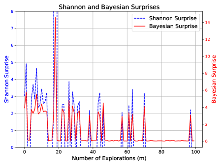
## Line Graph: Shannon and Bayesian Surprises
### Overview
The image is a line graph comparing two metrics, "Shannon Surprise" (blue dashed line) and "Bayesian Surprise" (red solid line), across a range of "Number of Explorations (m)" from 0 to 100. The graph highlights fluctuations in both metrics, with distinct peaks and troughs.
### Components/Axes
- **Title**: "Shannon and Bayesian Surprises" (top center).
- **X-axis**: "Number of Explorations (m)" with markers at 0, 20, 40, 60, 80, and 100.
- **Y-axes**:
- Left: "Shannon Surprise" (scale 0–8).
- Right: "Bayesian Surprise" (scale 0–14).
- **Legend**: Located in the top-right corner, associating:
- Blue dashed line → "Shannon Surprise".
- Red solid line → "Bayesian Surprise".
### Detailed Analysis
- **Shannon Surprise (Blue Dashed Line)**:
- Peaks at approximately **x = 20** (y ≈ 8), **x = 60** (y ≈ 6), and **x = 100** (y ≈ 4).
- Exhibits high variability, with sharp spikes and rapid declines.
- Smaller peaks observed near **x = 10** (y ≈ 5) and **x = 30** (y ≈ 3).
- **Bayesian Surprise (Red Solid Line)**:
- Peaks at approximately **x = 20** (y ≈ 12), **x = 60** (y ≈ 8), and **x = 100** (y ≈ 2).
- Smoother trend with less variability compared to Shannon Surprise.
- Smaller peaks near **x = 10** (y ≈ 4) and **x = 30** (y ≈ 2).
### Key Observations
1. **Peak Alignment**: Both metrics peak at similar x-values (20, 60, 100), suggesting correlated events or thresholds.
2. **Magnitude Difference**: Bayesian Surprise consistently exceeds Shannon Surprise in magnitude (e.g., 12 vs. 8 at x = 20).
3. **Volatility**: Shannon Surprise shows sharper fluctuations, while Bayesian Surprise remains relatively stable.
4. **Troughs**: Both metrics dip to near-zero values between peaks (e.g., x = 40–50, x = 80–90).
### Interpretation
The graph demonstrates that **Bayesian Surprise** consistently registers higher values than **Shannon Surprise**, indicating a potentially more sensitive or robust measure of surprise in this context. The alignment of peaks suggests shared underlying factors driving both metrics, such as critical exploration milestones. The volatility in Shannon Surprise may reflect its reliance on entropy-based calculations, which are more sensitive to discrete changes, whereas Bayesian Surprise’s smoother trend could imply probabilistic modeling that averages out noise. The troughs between peaks might represent periods of stability or predictable outcomes. This comparison could inform decisions in fields like machine learning or information theory, where balancing sensitivity and stability is critical.