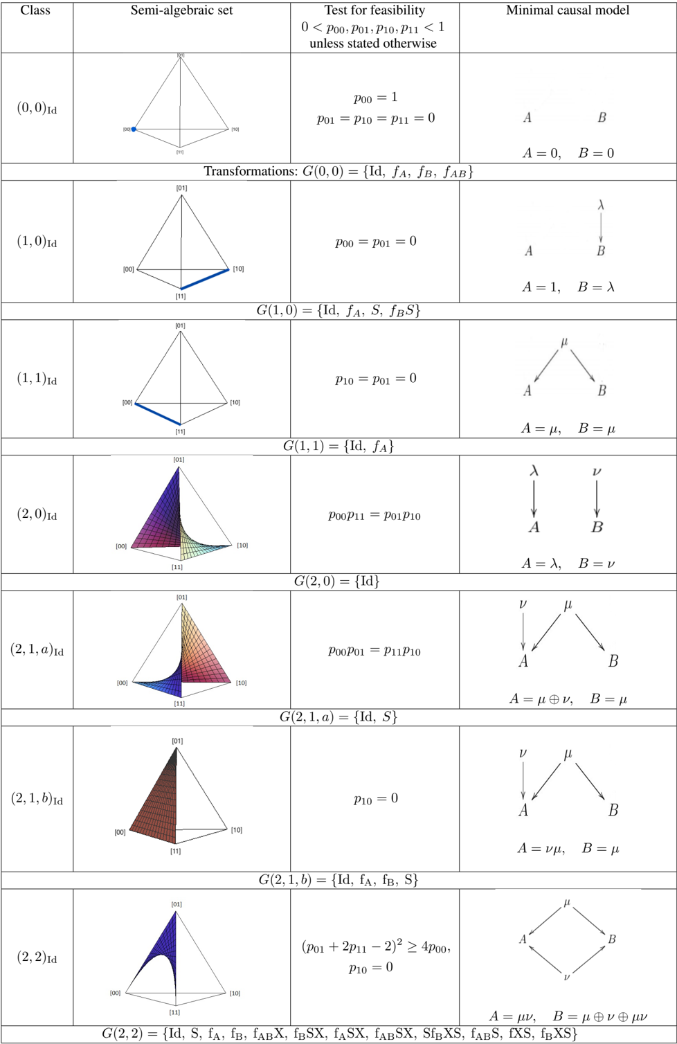
\n ## Table: Classification of Semi-Algebraic Sets and Minimal Causal Models for Binary Variables ### Overview The image displays a technical table classifying different "Classes" of statistical or causal models involving two binary variables (likely A and B). Each class is defined by a unique combination of a geometric representation (a semi-algebraic set within a probability tetrahedron), a mathematical feasibility test involving joint probabilities, and a corresponding minimal causal model depicted as a directed graph. The table is structured in four columns and eight primary rows, with each row separated by a horizontal line and often followed by a line specifying a group of transformations, `G(...)`. ### Components/Axes The table has four column headers: 1. **Class**: A label, e.g., `(0,0)Id`, `(1,0)Id`, `(2,1,a)Id`. 2. **Semi-algebraic set**: A 3D diagram of a tetrahedron with vertices labeled `[00]`, `[01]`, `[10]`, `[11]`. These vertices represent the four possible joint outcomes of two binary variables (e.g., A=0,B=0; A=0,B=1; etc.). The tetrahedron is the space of all possible joint probability distributions for these outcomes. Within each tetrahedron, a specific region, line, or point is highlighted (colored or shaded) to represent the set of distributions belonging to that class. 3. **Test for feasibility**: A mathematical condition on the joint probabilities `p00, p01, p10, p11`. The header states a general constraint: `0 < p00, p01, p10, p11 < 1 unless stated otherwise`. 4. **Minimal causal model**: A small directed acyclic graph (DAG) showing causal relationships between variables `A` and `B`, often involving latent variables (Greek letters). Below each graph is an equation defining `A` and `B` in terms of these variables and operations (e.g., `A = λ`, `B = μ ⊕ ν`). Between the rows for different classes, there are lines specifying a group of transformations, denoted as `G(class) = { ... }`. These likely represent symmetries or operations that map the model onto itself. ### Detailed Analysis The table is processed row by row, from top to bottom. **Row 1: Class (0,0)Id** * **Semi-algebraic set**: A tetrahedron with a single blue dot at vertex `[00]`. * **Test for feasibility**: `p00 = 1` and `p01 = p10 = p11 = 0`. This represents a deterministic distribution where only outcome (0,0) occurs. * **Minimal causal model**: Two independent nodes, `A` and `B`, with no arrows. `A = 0`, `B = 0`. This is a model of two constant, independent variables. * **Transformations**: `G(0,0) = {Id, f_A, f_B, f_AB}`. **Row 2: Class (1,0)Id** * **Semi-algebraic set**: A tetrahedron with a thick blue line connecting vertices `[11]` and `[10]`. * **Test for feasibility**: `p00 = p01 = 0`. This means outcomes where A=0 are impossible. * **Minimal causal model**: A latent variable `λ` points to `B`. `A` is independent. `A = 1`, `B = λ`. This suggests A is constant (1), and B is determined by a latent factor. * **Transformations**: `G(1,0) = {Id, f_A, S, f_BS}`. **Row 3: Class (1,1)Id** * **Semi-algebraic set**: A tetrahedron with a thick blue line connecting vertices `[00]` and `[11]`. * **Test for feasibility**: `p10 = p01 = 0`. This means the outcomes (1,0) and (0,1) are impossible; A and B always take the same value. * **Minimal causal model**: A latent variable `μ` points to both `A` and `B`. `A = μ`, `B = μ`. This is a model of perfect correlation due to a common cause. * **Transformations**: `G(1,1) = {Id, f_A}`. **Row 4: Class (2,0)Id** * **Semi-algebraic set**: A tetrahedron with a curved, shaded surface (gradient from purple at `[00]` to green at `[10]`) connecting vertices `[00]`, `[01]`, and `[10]`. The region is bounded by the edges from `[00]` to `[01]` and `[00]` to `[10]`. * **Test for feasibility**: `p00 * p11 = p01 * p10`. This is the condition for statistical independence between A and B. * **Minimal causal model**: Two independent latent variables, `λ` pointing to `A` and `ν` pointing to `B`. `A = λ`, `B = ν`. This is the classic model of independent causes. * **Transformations**: `G(2,0) = {Id}`. **Row 5: Class (2,1,a)Id** * **Semi-algebraic set**: A tetrahedron with a curved, shaded surface (gradient from blue at `[00]` to red at `[10]`) connecting vertices `[00]`, `[01]`, and `[10]`. The curvature appears different from the (2,0)Id case. * **Test for feasibility**: `p00 * p01 = p11 * p10`. * **Minimal causal model**: A latent variable `ν` points to `A`. Another latent variable `μ` points to both `A` and `B`. `A = μ ⊕ ν` (where `⊕` likely denotes XOR or addition mod 2), `B = μ`. This is a model where B is a cause of A, but A also has an independent cause. * **Transformations**: `G(2,1,a) = {Id, S}`. **Row 6: Class (2,1,b)Id** * **Semi-algebraic set**: A tetrahedron with a flat, shaded red triangle filling the face defined by vertices `[00]`, `[01]`, and `[11]`. * **Test for feasibility**: `p10 = 0`. Outcome (1,0) is impossible. * **Minimal causal model**: A latent variable `ν` points to `A`. A latent variable `μ` points to both `A` and `B`. `A = νμ` (product), `B = μ`. This is a different parametrization of a model where B influences A. * **Transformations**: `G(2,1,b) = {Id, f_A, f_B, S}`. **Row 7: Class (2,2)Id** * **Semi-algebraic set**: A tetrahedron with a curved, shaded blue surface connecting vertices `[00]`, `[01]`, and `[10]`. The shape is distinct from the previous curved surfaces. * **Test for feasibility**: `(p01 + 2p11 - 2)^2 >= 4p00` and `p10 = 0`. * **Minimal causal model**: A diamond-shaped graph. Latent variables `μ` and `ν` both point to `A` and `B`. `A = μν`, `B = μ ⊕ ν ⊕ μν`. This represents a more complex latent variable model. * **Transformations**: `G(2,2) = {Id, S, f_A, f_B, f_ABX, f_BSX, f_ASX, f_ABSX, Sf_BXS, f_ABS, fXS, f_BXS}`. This is the largest transformation group listed. ### Key Observations 1. **Geometric Progression**: The "Semi-algebraic set" column shows a clear progression from a point (0D), to a line (1D), to a surface (2D) within the 3D probability tetrahedron. The dimensionality of the set corresponds to the number of free parameters in the model. 2. **Feasibility Conditions**: The mathematical tests become more complex as the class number increases, moving from simple equalities (`p00=1`) to products (`p00*p11 = p01*p10`) and finally to inequalities involving squares. 3. **Causal Complexity**: The "Minimal causal model" graphs evolve from no connections, to single arrows, to common causes, to models with both direct and indirect influences, culminating in the diamond structure for class (2,2)Id. 4. **Transformation Groups**: The size of the transformation group `G` generally increases with the complexity of the class, suggesting more symmetries for more constrained models. Class (2,0)Id (independence) has only the identity transformation, indicating it is a unique, asymmetric point in the space of models. ### Interpretation This table provides a comprehensive taxonomy for the joint distribution of two binary variables from a causal inference perspective. Each "Class" represents a distinct **causal mechanism** or **generative model** that produces a specific family of probability distributions. * **The Tetrahedron**: It is the space of all possible joint distributions. The highlighted regions show which distributions are *compatible* with a given causal story. For example, the flat triangle in (2,1,b)Id (`p10=0`) represents all distributions where A and B are never (1,0). * **The Feasibility Test**: This is the **statistical signature** of the causal model. It's a necessary condition that data must satisfy to be explainable by that model. The condition `p00*p11 = p01*p10` is the well-known signature of independence. * **The Minimal Causal Model**: This is the **explanatory story**. It posits the simplest set of latent variables and direct causal links that could generate the observed statistical patterns. The equations (e.g., `A = μ ⊕ ν`) define how the observed variables are computed from the latent causes. * **The Transformations**: These represent **symmetries** of the model—operations (like flipping the value of A, `f_A`, or swapping A and B, `S`) that change the observed data but leave the underlying causal structure invariant. **In essence, the table maps causal explanations (right column) to their necessary statistical consequences (middle columns) within the geometric space of all possibilities (left column).** It is a foundational tool for understanding when observed data can or cannot be explained by a particular causal hypothesis about two binary variables. The progression illustrates how adding complexity to the causal story (more latent variables, more connections) allows it to explain a broader, more complex set of statistical patterns (higher-dimensional regions in the tetrahedron).