## Line Graphs: Cross Sections of J(x1, 0, ...) and J(0, x2, ...) in Dim 32
### Overview
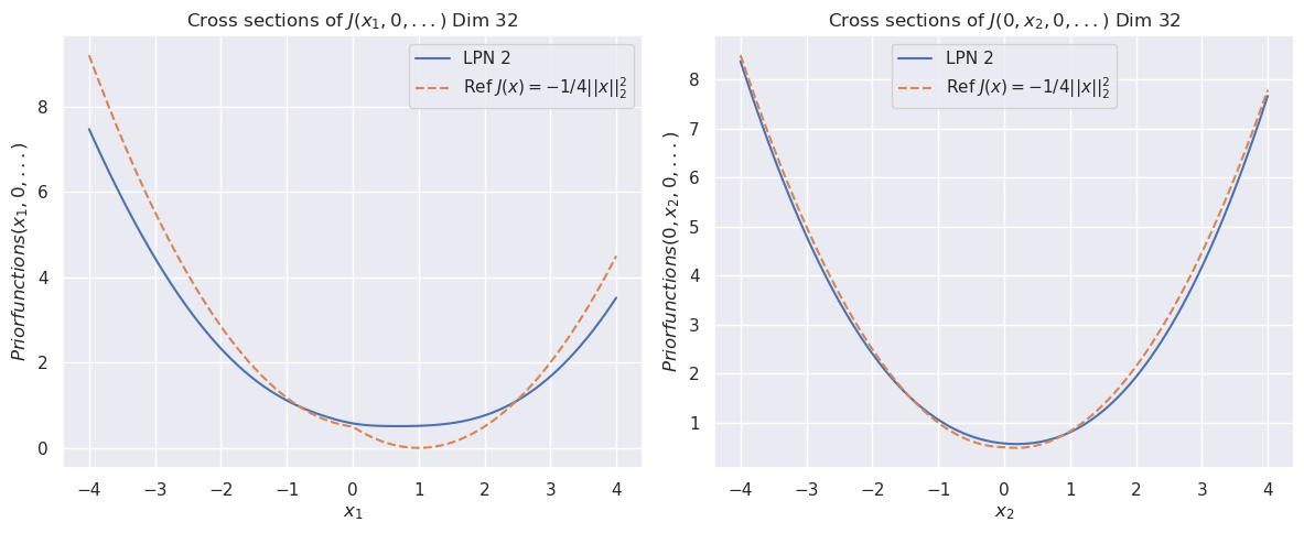
The image contains two side-by-side line graphs comparing prior functions for two cross-sections of a multidimensional function J. The left graph shows the cross-section along x₁ (with x₂=0, ...), and the right graph shows the cross-section along x₂ (with x₁=0, ...). Both graphs plot prior function values against their respective variables (x₁ or x₂) and include two data series: a solid blue line labeled "LPN 2" and a dashed red line labeled "Ref J(x) = -1/4||x||²".
### Components/Axes
- **Left Graph (x₁-axis):**
- **X-axis (x₁):** Ranges from -4 to 4 in increments of 1.
- **Y-axis (Priorfunctions(x₁, 0, ...)):** Ranges from 0 to 8 in increments of 1.
- **Legend:** Top-right corner, with blue for "LPN 2" and red dashed for "Ref J(x) = -1/4||x||²".
- **Right Graph (x₂-axis):**
- **X-axis (x₂):** Ranges from -4 to 4 in increments of 1.
- **Y-axis (Priorfunctions(0, x₂, 0, ...)):** Ranges from 1 to 8 in increments of 1.
- **Legend:** Top-right corner, same labels as the left graph.
### Detailed Analysis
#### Left Graph (x₁-axis):
- **LPN 2 (Blue Solid Line):**
- Starts at ~7.5 when x₁ = -4.
- Decreases smoothly to a minimum of ~0.5 at x₁ = 0.
- Increases back to ~7.5 at x₁ = 4.
- **Reference Function (Red Dashed Line):**
- Starts at ~8.5 when x₁ = -4.
- Decreases sharply to a minimum of ~0.25 at x₁ = 0.
- Increases back to ~8.5 at x₁ = 4.
#### Right Graph (x₂-axis):
- **LPN 2 (Blue Solid Line):**
- Starts at ~8 when x₂ = -4.
- Decreases smoothly to a minimum of ~0.25 at x₂ = 0.
- Increases back to ~8 at x₂ = 4.
- **Reference Function (Red Dashed Line):**
- Starts at ~8.5 when x₂ = -4.
- Decreases sharply to a minimum of ~0.25 at x₂ = 0.
- Increases back to ~8.5 at x₂ = 4.
### Key Observations
1. **Symmetry:** Both graphs exhibit symmetric behavior around x=0, consistent with the quadratic reference function J(x) = -1/4||x||².
2. **LPN 2 vs. Reference Function:**
- The LPN 2 line is consistently flatter and less steep than the reference function, suggesting a less restrictive prior.
- The reference function has a deeper minimum at x=0, indicating a stricter prior centered at the origin.
3. **Y-axis Discrepancy:** The right graph’s y-axis starts at 1, while the left starts at 0. This may reflect a scaling difference or a labeling error, as the LPN 2 line dips below 1 in the right graph (e.g., ~0.25 at x₂=0).
### Interpretation
- **Prior Function Behavior:** The graphs compare two prior distributions (LPN 2 and the reference function) in cross-sectional views of a 32-dimensional space. The reference function’s sharper minimum suggests it penalizes deviations from the origin more heavily, while LPN 2 allows broader variability.
- **Dimensionality Impact:** The consistent shape across x₁ and x₂ cross-sections implies the prior functions are isotropic (symmetric in all dimensions).
- **Anomaly:** The right graph’s y-axis starting at 1 conflicts with the LPN 2 line’s value of ~0.25 at x₂=0. This may indicate a plotting error or intentional scaling to emphasize certain features.
The data highlights trade-offs between strictness and flexibility in prior distributions, with implications for Bayesian modeling or optimization in high-dimensional spaces.