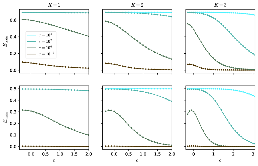
## Line Charts: Training Error (E_train) vs. Parameter (c) for Different Model Complexity (K) and Regularization (r) ### Overview The image displays a 2x3 grid of six line charts. The charts plot the training error, denoted as **E_train**, on the y-axis against a parameter **c** on the x-axis. Each column of charts corresponds to a different value of **K** (K=1, K=2, K=3), which likely represents model complexity or a similar hyperparameter. Within each chart, four distinct lines represent different values of a parameter **r** (r=10⁴, r=10², r=10⁰, r=10⁻²), which appears to be a regularization strength or a related coefficient. The overall visualization demonstrates how the training error evolves with the parameter `c` under varying conditions of model complexity (`K`) and regularization (`r`). ### Components/Axes * **Y-axis (All Charts):** Labeled **E_train**. Represents the training error metric. * Top Row Scale: Ranges from 0.0 to approximately 0.7. * Bottom Row Scale: Ranges from 0.0 to 0.5. * **X-axis (All Charts):** Labeled **c**. Represents an independent parameter. * Charts for K=1 and K=2: The x-axis ranges from 0.0 to 2.0. * Charts for K=3: The x-axis ranges from 0 to 3. * **Column Headers:** Each column is titled with the value of **K**. * Left Column: **K=1** * Middle Column: **K=2** * Right Column: **K=3** * **Legend (Present in the top-left chart, K=1):** Located in the center-left area of the plot. It defines the four data series by color and line style (solid line with circular markers). * **Cyan Line:** `r = 10⁴` * **Teal Line:** `r = 10²` * **Green Line:** `r = 10⁰` (which equals 1) * **Brown Line:** `r = 10⁻²` (which equals 0.01) ### Detailed Analysis The analysis is segmented by the `K` value (columns). **Column 1: K=1** * **Top Chart (E_train scale ~0-0.7):** * `r=10⁴` (Cyan): Nearly horizontal line at the top, E_train ≈ 0.7, showing almost no change as `c` increases. * `r=10²` (Teal): Starts at E_train ≈ 0.6, slopes gently downward to ≈ 0.4 at c=2.0. * `r=10⁰` (Green): Follows a nearly identical path to the teal line, starting at ≈ 0.6 and ending at ≈ 0.4. * `r=10⁻²` (Brown): Starts low at E_train ≈ 0.1, slopes gently downward to ≈ 0.05 at c=2.0. * **Bottom Chart (E_train scale 0-0.5):** * `r=10⁴` (Cyan): Nearly horizontal line at E_train ≈ 0.5. * `r=10²` (Teal): Starts at ≈ 0.32, slopes downward to ≈ 0.1 at c=2.0. * `r=10⁰` (Green): Follows a nearly identical path to the teal line. * `r=10⁻²` (Brown): A flat line very close to E_train = 0.0 across the entire range of `c`. **Column 2: K=2** * **Top Chart:** * `r=10⁴` (Cyan): Nearly horizontal at E_train ≈ 0.7. * `r=10²` (Teal): Starts at ≈ 0.6, curves downward more steeply than in K=1, reaching ≈ 0.15 at c=2.0. * `r=10⁰` (Green): Follows a nearly identical path to the teal line. * `r=10⁻²` (Brown): Starts at ≈ 0.1, slopes downward to near 0.0 at c=2.0. * **Bottom Chart:** * `r=10⁴` (Cyan): Nearly horizontal at E_train ≈ 0.5. * `r=10²` (Teal): Starts at ≈ 0.32, curves downward, approaching 0.0 at c=2.0. * `r=10⁰` (Green): Follows a nearly identical path to the teal line. * `r=10⁻²` (Brown): Flat line at E_train = 0.0. **Column 3: K=3** * **Top Chart (x-axis extends to 3):** * `r=10⁴` (Cyan): Nearly horizontal at E_train ≈ 0.7, with a very slight downward curve at the far right (c=3). * `r=10²` (Teal): Starts at ≈ 0.6, curves downward sharply, crossing below the green line around c=1.5 and reaching ≈ 0.2 at c=3. * `r=10⁰` (Green): Starts at ≈ 0.58, curves downward very steeply, approaching 0.0 by c=2.5. * `r=10⁻²` (Brown): Starts at ≈ 0.1, drops quickly to near 0.0 by c=1.0 and remains flat. * **Bottom Chart (x-axis extends to 3):** * `r=10⁴` (Cyan): Nearly horizontal at E_train ≈ 0.5, with a slight downward curve starting around c=2. * `r=10²` (Teal): Starts at ≈ 0.32, curves downward sharply, approaching 0.0 by c=3. * `r=10⁰` (Green): Starts at ≈ 0.3, exhibits a small local maximum (bump) around c=0.5, then plummets steeply to 0.0 by c=1.5. * `r=10⁻²` (Brown): Flat line at E_train = 0.0. ### Key Observations 1. **Effect of `r` (Regularization):** Higher values of `r` (10⁴, cyan) consistently result in higher training error (`E_train`) that is largely insensitive to changes in `c`. Lower values of `r` (10⁻², brown) lead to very low training error, often near zero. 2. **Effect of `K` (Complexity):** As `K` increases from 1 to 3, the curves for intermediate `r` values (10² and 10⁰) become steeper. The decline in `E_train` with increasing `c` happens more rapidly and reaches lower values for higher `K`. 3. **Interaction between `r` and `c`:** For a fixed `K`, the parameter `c` has a much stronger effect on reducing `E_train` for intermediate `r` values (10², 10⁰) than for the very high or very low `r` extremes. 4. **Convergence:** For `K=2` and `K=3`, the lines for `r=10²` and `r=10⁰` converge to similar low error values as `c` increases, especially in the bottom row of charts. 5. **Anomaly:** In the bottom chart for K=3, the green line (`r=10⁰`) shows a distinct non-monotonic behavior with a local peak around c=0.5 before its steep descent. ### Interpretation This set of charts likely illustrates the bias-variance trade-off or the effect of regularization in a machine learning context. `E_train` is the error on the training dataset. * **High `r` (Strong Regularization):** The model is heavily constrained (high bias). It cannot fit the training data well, resulting in high `E_train` that doesn't improve much with the tuning parameter `c`. The model is underfitting. * **Low `r` (Weak Regularization):** The model is very flexible (low bias). It can fit the training data almost perfectly (`E_train ≈ 0`), regardless of `c`. This risks overfitting, though only training error is shown here. * **Intermediate `r`:** This is the interesting regime. Here, the parameter `c` acts as a crucial tuning knob. Increasing `c` systematically reduces the training error, and this effect is amplified with greater model complexity (`K`). The steep descent suggests that for these regularization strengths, the model's capacity to learn from the data is highly sensitive to `c`. * **Role of `K`:** Increasing `K` (model complexity) makes the model more responsive to the parameter `c` when regularization is not too strong. The sharper declines for K=3 indicate that a more complex model can leverage the adjustment provided by `c` to reduce training error more effectively, but this also heightens the risk of overfitting if validation error were plotted. In summary, the visualization demonstrates that optimal model performance (balancing fit and generalization) would likely be found by selecting an intermediate `r` and then tuning `c`, with the optimal `c` value potentially depending on the chosen model complexity `K`. The charts provide a clear map of how these three hyperparameters interact to influence training error.