## Line Chart: Invariance Penalty vs. Weight of $\Phi$
### Overview
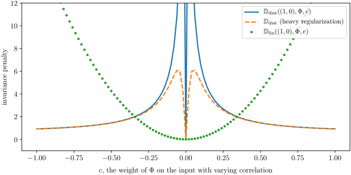
This image displays a line chart illustrating the relationship between the "invariance penalty" (y-axis) and "$c$, the weight of $\Phi$ on the input with varying correlation" (x-axis). The chart compares three distinct mathematical functions, likely representing different regularization or distance metrics used in machine learning optimization (specifically related to Invariant Risk Minimization or similar domain generalization frameworks). The chart demonstrates how these penalties behave as the correlation weight $c$ moves from -1.0 to 1.0.
The language used in the chart is English, accompanied by standard mathematical notation.
### Components/Axes
* **X-Axis:** Labeled "$c$, the weight of $\Phi$ on the input with varying correlation". The scale ranges from -1.00 to 1.00, with major ticks every 0.25.
* **Y-Axis:** Labeled "invariance penalty". The scale ranges from 0 to 12, with major ticks every 2 units.
* **Legend:** Located in the top-right quadrant of the chart area.
* **Solid Blue Line:** $\mathbb{D}_{\text{dist}}((1, 0), \Phi, e)$
* **Dashed Orange Line:** $\mathbb{D}_{\text{dist}}$ (heavy regularization)
* **Green Dotted Line:** $\mathbb{D}_{\text{lin}}((1, 0), \Phi, e)$
### Detailed Analysis
#### 1. Solid Blue Line: $\mathbb{D}_{\text{dist}}((1, 0), \Phi, e)$
* **Trend:** This line exhibits a sharp, asymptotic spike at $c = 0$. As $|c|$ increases away from 0, the penalty drops precipitously.
* **Values:**
* At $c = 0$, the value approaches infinity (exits the top of the chart).
* At $c = \pm 0.25$, the value is approximately 2.0.
* At $c = \pm 0.50$, the value is approximately 1.5.
* At $c = \pm 1.00$, the value flattens out near 1.0.
#### 2. Dashed Orange Line: $\mathbb{D}_{\text{dist}}$ (heavy regularization)
* **Trend:** This line follows a similar trajectory to the solid blue line at the extremes ($|c| > 0.25$), but behaves differently near the origin. It exhibits a sharp, narrow spike at $c=0$, but with a lower peak than the blue line. It appears to have local maxima (peaks) at approximately $c = \pm 0.05$ with a value of roughly 6.0.
* **Values:**
* At $c = 0$, the value drops to near 0.
* At $c = \pm 0.05$, the value peaks at approximately 6.0.
* At $c = \pm 0.25$, the value is approximately 2.0 (converging with the blue line).
* At $c = \pm 1.00$, the value flattens out near 1.0.
#### 3. Green Dotted Line: $\mathbb{D}_{\text{lin}}((1, 0), \Phi, e)$
* **Trend:** This line follows a parabolic, U-shaped curve. It is symmetric around the y-axis.
* **Values:**
* At $c = 0$, the value is 0.0 (the global minimum).
* At $c = \pm 0.25$, the value is approximately 1.0.
* At $c = \pm 0.50$, the value is approximately 3.5.
* At $c = \pm 0.75$, the value is approximately 9.0.
* At $c = \pm 1.00$, the value exceeds 12.0.
### Key Observations
* **Symmetry:** All three functions are symmetric around $c = 0$.
* **Inverse Relationship:** The Green Dotted Line ($\mathbb{D}_{\text{lin}}$) is essentially the inverse of the distance-based metrics ($\mathbb{D}_{\text{dist}}$) in terms of penalty distribution. While the distance metrics penalize the origin ($c=0$) heavily, the linear metric rewards the origin with a zero penalty.
* **Regularization Effect:** The "heavy regularization" (orange dashed line) effectively "clips" or modifies the behavior of the standard distance metric (blue line) near the origin, creating a distinct local peak rather than a pure asymptotic spike.
### Interpretation
This chart visualizes the "Invariance Penalty" landscape for different loss functions.
* **The Distance Metrics ($\mathbb{D}_{\text{dist}}$):** These functions appear designed to penalize models that rely on specific correlations (where $c$ is near 0). The "heavy regularization" variant suggests a technique used to stabilize training or prevent the penalty from becoming numerically unstable (exploding gradients) at the origin, though it introduces a complex landscape with local maxima near $c=0$.
* **The Linear Metric ($\mathbb{D}_{\text{lin}}$):** This function acts as a standard convex loss, where the penalty increases as the weight $c$ deviates from the ideal state of 0.
* **Implications:** The chart demonstrates a trade-off. If the goal is to enforce invariance (where $c=0$ is the target), the $\mathbb{D}_{\text{dist}}$ metrics create a very steep "cliff" that forces the model away from $c=0$ unless it is perfectly invariant. The "heavy regularization" is likely a practical implementation to make this optimization landscape more tractable by smoothing the spike at the origin.