## Diagram: Hexagonal Packing ### Overview The image shows two separate diagrams, each depicting a hexagonal shape filled with smaller, blue hexagonal shapes. The larger hexagonal shapes are outlined in red. The arrangement of the smaller hexagons differs between the two diagrams, suggesting different packing configurations. ### Components/Axes * **Outer Shape:** Red hexagon. * **Inner Shapes:** Blue hexagons. * **Arrangement:** Two different arrangements of the blue hexagons within the red hexagon. ### Detailed Analysis **Left Diagram:** * Contains 11 complete blue hexagons and 1 partial hexagon. * The blue hexagons are arranged somewhat randomly, with some gaps and overlaps. * The partial hexagon is located on the right side of the red hexagon. **Right Diagram:** * Contains 12 complete blue hexagons. * The blue hexagons are arranged in a more organized, close-packed manner. * There are fewer gaps between the blue hexagons compared to the left diagram. ### Key Observations * The two diagrams illustrate different ways to pack smaller hexagons within a larger hexagon. * The right diagram appears to represent a more efficient packing arrangement, as it contains more complete hexagons and fewer gaps. ### Interpretation The image likely demonstrates different packing densities or arrangements of hexagonal units within a confined hexagonal space. The right diagram suggests a more optimized or efficient packing strategy compared to the left diagram. This could be relevant in fields like materials science, where the arrangement of atoms or molecules can affect the properties of a material. The diagrams do not provide specific data, but rather a visual comparison of two different configurations.

\n ## Diagram: Hexagonal Packing Comparison ### Overview The image presents a visual comparison of two hexagonal packing arrangements within larger hexagonal boundaries. The left arrangement contains fewer hexagons, while the right arrangement contains more, demonstrating a difference in packing density. There are no labels, axes, or legends present. ### Components/Axes The image consists of: * **Large Hexagon:** A red outline forming the boundary for each arrangement. * **Small Hexagons:** Blue filled hexagons arranged within the larger hexagon. * **Arrangement 1 (Left):** Contains approximately 10-12 small hexagons. * **Arrangement 2 (Right):** Contains approximately 18-20 small hexagons. ### Detailed Analysis or Content Details The image does not contain numerical data or specific measurements. The analysis is based on visual counting and estimation. * **Arrangement 1:** The small hexagons are arranged in a less organized manner, with more empty space between them. The arrangement appears somewhat random. * **Arrangement 2:** The small hexagons are arranged in a more regular, tightly packed pattern. The arrangement appears more organized and efficient in terms of space utilization. * The large hexagons appear to be of similar size in both arrangements. ### Key Observations The primary observation is the difference in the number of small hexagons that can be packed within the same-sized large hexagon, indicating a difference in packing efficiency. Arrangement 2 demonstrates a higher packing density than Arrangement 1. ### Interpretation The image illustrates the concept of hexagonal close packing. Hexagonal packing is an efficient way to fill a plane with equal-sized circles (or in this case, hexagons). The right arrangement demonstrates a more optimal packing configuration, maximizing the number of hexagons within the given area. This is a fundamental concept in materials science, chemistry (e.g., crystal structures), and geometry. The difference between the two arrangements highlights how the arrangement of elements can significantly impact density and space utilization. The image does not provide any quantitative data, but serves as a qualitative demonstration of the principle.

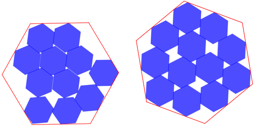
## Diagram: Hexagonal Packing Efficiency Comparison ### Overview The image displays two side-by-side diagrams illustrating different arrangements of identical blue hexagons within irregular red polygonal boundaries. The diagram on the left shows a loose, inefficient packing with significant gaps, while the diagram on the right shows a tight, efficient packing with minimal gaps. There is no textual information, labels, axes, or legends present in the image. ### Components/Axes * **Primary Components:** * **Blue Hexagons:** Solid blue, regular hexagons of uniform size and orientation. * **Red Boundary Lines:** Thin red lines forming irregular, non-convex polygons that enclose the hexagons. * **Spatial Layout:** Two distinct clusters are presented horizontally. The left cluster is labeled here as "Diagram A" and the right as "Diagram B" for reference. * **Text/Labels:** None present. The image is purely graphical. ### Detailed Analysis **Diagram A (Left):** * **Arrangement:** Contains 11 blue hexagons arranged in a loose, irregular cluster. * **Packing Efficiency:** Low. There are large, irregular white gaps between many of the hexagons. The hexagons do not share edges consistently, and their centers are not aligned in a regular lattice. * **Boundary Fit:** The red boundary line loosely follows the outer perimeter of the cluster, with significant empty space between the hexagons and the boundary in several areas, particularly at the top and bottom. **Diagram B (Right):** * **Arrangement:** Contains 13 blue hexagons arranged in a tight, regular pattern. * **Packing Efficiency:** High. The hexagons are arranged in a classic hexagonal (honeycomb) tessellation. Each internal hexagon shares edges with six neighbors, leaving only small, triangular gaps at the junctions of three hexagons. * **Boundary Fit:** The red boundary line closely follows the outer perimeter of the tightly packed cluster. The fit is much snugger compared to Diagram A, with minimal wasted space between the hexagons and the boundary. ### Key Observations 1. **Density Contrast:** The most striking observation is the dramatic difference in packing density between the two arrangements. Diagram B contains more hexagons (13 vs. 11) within a visually similar total area defined by the red boundary. 2. **Geometric Order vs. Disorder:** Diagram A represents a disordered, random packing state. Diagram B represents an ordered, crystalline packing state. 3. **Boundary Interaction:** The irregular red boundary in Diagram A appears to constrain a disordered system inefficiently. In Diagram B, the same style of boundary tightly contains an ordered system that maximizes the use of the available space. ### Interpretation This diagram is a visual metaphor for the concept of **packing efficiency** or **spatial optimization**. It demonstrates a fundamental principle in geometry, materials science, logistics, and nature: * **What it suggests:** The data (visual arrangement) suggests that ordered, tessellating patterns (like the hexagonal lattice in B) achieve significantly higher density and material utilization than disordered arrangements (A) of the same components. * **How elements relate:** The red boundary represents a fixed container or constrained area. The blue hexagons represent discrete units (atoms, molecules, packages, cells). The relationship shows how the *arrangement* of units within a container drastically affects the total capacity and efficiency. * **Notable Anomalies/Trends:** The "anomaly" is the inefficiency of Diagram A. The clear trend is toward order (B) as the optimal solution for maximizing the number of units within a given space. This principle explains why honeycombs are structurally efficient, why crystals form regular lattices, and why hexagonal grids are used in warehouse planning and computational geometry. **In essence, the image communicates that structure and order are key to efficiency in spatial packing problems.**

## Diagram: Hexagonal Grid Configurations ### Overview The image displays two side-by-side hexagonal grids, each enclosed by a red outline. Both grids contain smaller blue hexagons arranged within the larger red hexagon. The left grid shows a clustered arrangement of blue hexagons, while the right grid exhibits a more uniform, grid-like pattern. ### Components/Axes - **Primary Elements**: - Two red hexagonal boundaries (left and right). - Blue hexagons nested within each red hexagon. - **Spatial Relationships**: - Left grid: Blue hexagons are densely packed with irregular spacing. - Right grid: Blue hexagons are evenly distributed with consistent gaps. - **No textual labels, legends, or axis markers are present.** ### Detailed Analysis - **Left Grid**: - Contains **12 blue hexagons**. - Arrangement: Irregular clustering, with some hexagons overlapping or partially obscured by others. - Gaps: Irregularly shaped white spaces between blue hexagons. - **Right Grid**: - Contains **15 blue hexagons**. - Arrangement: Uniform grid pattern, with hexagons aligned in rows and columns. - Gaps: Symmetrical white spaces between hexagons. ### Key Observations 1. **Quantity Difference**: The right grid holds 3 more blue hexagons than the left. 2. **Structural Contrast**: - Left grid emphasizes density and irregularity. - Right grid emphasizes uniformity and symmetry. 3. **Boundary Consistency**: Both red hexagons are identical in size and shape, suggesting a controlled comparison. ### Interpretation The diagram likely illustrates a comparison of hexagonal tiling strategies. The left grid’s clustered arrangement could represent a scenario prioritizing space efficiency (e.g., packing), while the right grid’s uniform layout might reflect optimization for accessibility or modularity. The absence of labels or legends leaves the exact purpose ambiguous, but the visual contrast suggests a focus on geometric efficiency versus structural regularity. **Note**: No textual data or numerical values are present in the image. All observations are based on spatial and quantitative analysis of the hexagons’ arrangement.