\n
## Line Graph: Convergence of Trace Estimators
### Overview
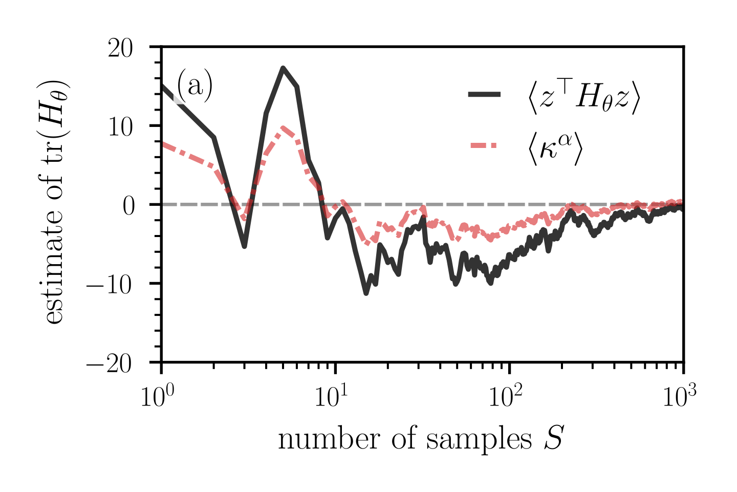
The image displays a scientific line graph comparing two different estimators for the trace of a Hessian matrix, `tr(H_θ)`, as a function of the number of samples, `S`. The plot demonstrates the convergence behavior and variance of these estimators. The label "(a)" in the top-left corner indicates this is likely panel (a) of a larger multi-part figure.
### Components/Axes
* **Y-Axis:**
* **Label:** `estimate of tr(H_θ)`
* **Scale:** Linear, ranging from -20 to 20.
* **Ticks:** Major ticks at intervals of 10 (-20, -10, 0, 10, 20). Minor ticks are present between major ticks.
* **X-Axis:**
* **Label:** `number of samples S`
* **Scale:** Logarithmic (base 10).
* **Range:** From `10^0` (1) to `10^3` (1000).
* **Ticks:** Major ticks at `10^0`, `10^1`, `10^2`, `10^3`. Minor ticks are present between major ticks.
* **Legend:**
* **Position:** Top-right quadrant of the plot area.
* **Entry 1:** A solid black line, labeled with the mathematical expression `⟨z^T H_θ z⟩`.
* **Entry 2:** A dashed pink/salmon-colored line, labeled with the mathematical expression `⟨κ^α⟩`.
* **Reference Line:** A dashed gray horizontal line is drawn at `y = 0`.
### Detailed Analysis
The graph plots two data series against the logarithmic sample size `S`.
1. **Series `⟨z^T H_θ z⟩` (Solid Black Line):**
* **Trend:** Starts at a high positive value, exhibits large oscillations for small `S`, and gradually converges toward zero with decreasing variance as `S` increases.
* **Approximate Data Points:**
* At `S = 1` (`10^0`): y ≈ 15.
* At `S ≈ 2`: y drops sharply to a local minimum ≈ -5.
* At `S ≈ 5-6`: y peaks at a global maximum ≈ 18.
* At `S ≈ 10` (`10^1`): y is near 0.
* For `S > 10`: The line fluctuates significantly below zero, reaching a minimum near -12 around `S ≈ 20-30`. It then trends upward, crossing zero around `S ≈ 200`, and continues to oscillate with decreasing amplitude around zero up to `S = 1000`.
2. **Series `⟨κ^α⟩` (Dashed Pink Line):**
* **Trend:** Follows a pattern qualitatively similar to the black line but with consistently smaller amplitude (lower variance). It also converges toward zero as `S` increases.
* **Approximate Data Points:**
* At `S = 1`: y ≈ 8.
* At `S ≈ 2`: y drops to a local minimum ≈ -2.
* At `S ≈ 5-6`: y peaks at ≈ 10.
* At `S ≈ 10`: y is near 0.
* For `S > 10`: The line fluctuates mostly between -5 and 0, trending upward and converging to zero from below. By `S = 1000`, it is very close to zero.
### Key Observations
* **High Initial Variance:** Both estimators show extremely high variance and bias for very small sample sizes (`S < 10`), with values swinging from large positive to negative.
* **Convergence:** Both series clearly converge toward the reference line at `y = 0` as the number of samples `S` increases. The convergence appears to be in the mean, with the oscillations dampening.
* **Relative Performance:** The estimator `⟨κ^α⟩` (pink dashed) exhibits lower variance (smaller oscillations) than `⟨z^T H_θ z⟩` (black solid) across the entire range of `S`, particularly for `S < 100`.
* **Bias at Low S:** For small `S`, both estimators appear to have a positive bias (starting above zero), which then reverses into a negative bias for intermediate `S` (roughly 10 to 100) before converging.
### Interpretation
This graph is a diagnostic tool comparing the statistical efficiency of two methods for estimating the trace of a Hessian matrix, a quantity important in optimization and machine learning (e.g., for understanding loss landscape curvature or computing the Fisher information matrix).
* **What the data suggests:** The plot demonstrates that both proposed estimators are *consistent*—their expected value converges to the true value (presumably zero in this test case) as the sample size `S` grows. However, they differ significantly in their *variance*.
* **Relationship between elements:** The `⟨κ^α⟩` estimator appears to be a variance-reduced version of the `⟨z^T H_θ z⟩` estimator. The similar shape of the curves suggests they are estimating the same underlying quantity, but the pink dashed line's tighter oscillations indicate it is a more statistically efficient estimator, requiring fewer samples to achieve a given level of precision.
* **Notable Anomalies/Trends:** The most striking feature is the dramatic reduction in variance for both estimators once `S` exceeds approximately 100. This suggests a phase transition in the estimation error, where the law of large numbers begins to dominate. The initial positive bias and subsequent negative bias for intermediate `S` could be indicative of properties of the specific distribution from which the samples `z` are drawn or the geometry of the Hessian `H_θ` at the point of estimation.
**In summary, the image provides empirical evidence that the estimator `⟨κ^α⟩` offers a more stable and precise approximation of `tr(H_θ)` than the `⟨z^T H_θ z⟩` estimator, especially in the computationally constrained regime of a low number of samples.**