# Technical Data Extraction: Conductance Plots (a) and (b)
This document provides a comprehensive extraction of the data and components from the provided image, which consists of two side-by-side line charts representing conductance ($G$) as a function of Rashba coupling ($\lambda_R/t$).
## 1. Global Metadata and Axis Definitions
* **Y-Axis (Primary):** Conductance $G$ measured in units of $(e^2/\hbar)$.
* **Scale:** 0 to 3.5.
* **Major Tick Marks:** 0, 1, 2, 3.
* **X-Axis (Primary):** Dimensionless Rashba coupling parameter $\lambda_R/t$.
* **Scale:** 0.00 to 0.25.
* **Major Tick Marks:** 0.00, 0.05, 0.10, 0.15, 0.20, 0.25.
* **Visual Features:** Both plots contain a light gray shaded horizontal band between $G \approx 0$ and $G \approx 1.5$.
---
## 2. Panel (a) Analysis
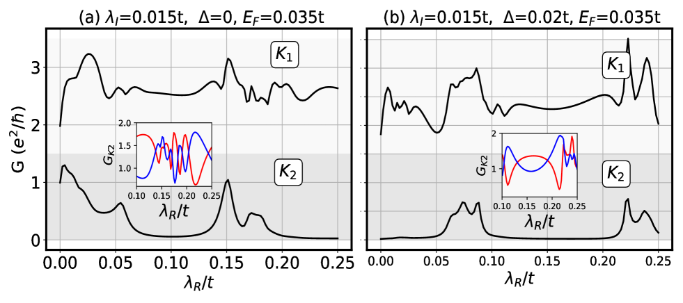
**Header Label:** (a) $\lambda_I = 0.015t, \Delta = 0, E_F = 0.035t$
### Main Plot Components
Panel (a) contains two distinct black data series labeled with boxed text.
* **Series $K_1$ (Upper Line):**
* **Trend:** Starts at $G \approx 2.0$. It shows a significant peak at $\lambda_R/t \approx 0.025$ reaching $G \approx 3.2$. It then oscillates with a general downward trend toward $G \approx 2.5$ before a sharp spike at $\lambda_R/t \approx 0.15$ (reaching $G \approx 3.1$). It ends at $G \approx 2.6$.
* **Spatial Grounding:** Label $K_1$ is located at the top right [x=0.85, y=0.90] relative to the panel.
* **Series $K_2$ (Lower Line):**
* **Trend:** Starts at $G \approx 1.0$, peaks quickly at $\lambda_R/t \approx 0.01$, then decays toward zero. It remains near zero between $0.07 < \lambda_R/t < 0.13$. It exhibits a sharp, narrow peak at $\lambda_R/t \approx 0.15$ (reaching $G \approx 1.0$) and then returns to near zero.
* **Spatial Grounding:** Label $K_2$ is located at the middle right [x=0.85, y=0.40] relative to the panel.
### Inset Plot (a)
* **Axes:** Y-axis is $G_{K2}$ (range 0.5 to 2.0); X-axis is $\lambda_R/t$ (range 0.10 to 0.25).
* **Data Series:**
* **Blue Line:** Starts low ($\approx 0.8$), rises to a peak at $\approx 0.22$, then drops.
* **Red Line:** Starts high ($\approx 1.7$), drops to a minimum at $\approx 0.22$, then rises.
* **Observation:** The blue and red lines show an anti-correlated oscillatory behavior.
---
## 3. Panel (b) Analysis
**Header Label:** (b) $\lambda_I = 0.015t, \Delta = 0.02t, E_F = 0.035t$
*Note: The introduction of $\Delta = 0.02t$ is the primary variable change from panel (a).*
### Main Plot Components
* **Series $K_1$ (Upper Line):**
* **Trend:** Starts at $G \approx 1.8$. It shows a series of small oscillations between $0.00 < \lambda_R/t < 0.05$, a dip at $0.05$, and a broad plateau around $G \approx 2.3$. A very sharp, high-amplitude double peak occurs between $0.20 < \lambda_R/t < 0.25$, with the highest point reaching $G \approx 3.5$.
* **Spatial Grounding:** Label $K_1$ is located at [x=0.85, y=0.85].
* **Series $K_2$ (Lower Line):**
* **Trend:** Remains at $G \approx 0$ for the majority of the range. It shows a small double-hump feature between $0.06 < \lambda_R/t < 0.10$ (max $G \approx 0.7$). It returns to zero and then shows a final sharp peak at $\lambda_R/t \approx 0.22$ (max $G \approx 0.8$).
* **Spatial Grounding:** Label $K_2$ is located at [x=0.85, y=0.40].
### Inset Plot (b)
* **Axes:** Y-axis is $G_{K2}$ (range 0 to 2); X-axis is $\lambda_R/t$ (range 0.10 to 0.25).
* **Data Series:**
* **Blue Line:** Shows a "W" shape; peaks at $0.11$ and $0.22$, with a local minimum in the center.
* **Red Line:** Shows an "M" shape; peaks in the center ($\lambda_R/t \approx 0.17$) and has deep minima at $0.11$ and $0.22$.
* **Observation:** These lines are perfectly out of phase (anti-correlated).
---
## 4. Summary of Key Trends
1. **Effect of $\Delta$:** Comparing (a) to (b), the introduction of a non-zero $\Delta$ suppresses the conductance of $K_2$ across most of the $\lambda_R/t$ range, except for specific resonance peaks.
2. **Resonance:** Both plots show sharp conductance spikes at high $\lambda_R/t$ values (around 0.15 for $\Delta=0$ and around 0.22 for $\Delta=0.02t$).
3. **Symmetry in Insets:** The insets reveal that while the total conductance might fluctuate, the sub-components (Red and Blue lines) maintain a reciprocal relationship, where the increase in one corresponds to the decrease in the other.