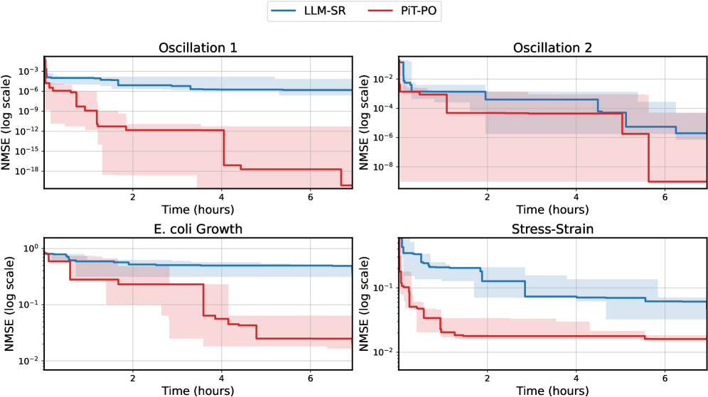
## Line Chart Comparison: NMSE vs. Time for Two Methods ### Overview The image displays a 2x2 grid of four line charts comparing the performance of two methods, **LLM-SR** (blue line) and **PiT-PO** (red line), across four different tasks or datasets. Performance is measured by **Normalized Mean Squared Error (NMSE)** on a logarithmic scale over **Time (hours)**. Each chart includes shaded regions around the main lines, likely representing confidence intervals or standard deviation. ### Components/Axes * **Legend:** Located at the top center of the entire figure. It defines: * **Blue Line:** LLM-SR * **Red Line:** PiT-PO * **Common Axes (All Subplots):** * **X-axis:** Label: "Time (hours)". Scale: Linear, from 0 to approximately 7 hours. Major ticks at 0, 2, 4, 6. * **Y-axis:** Label: "NMSE (log scale)". Scale: Logarithmic. The range varies per subplot. * **Subplot Titles (Top Center of each chart):** 1. Top-Left: **Oscillation 1** 2. Top-Right: **Oscillation 2** 3. Bottom-Left: **E. coli Growth** 4. Bottom-Right: **Stress-Strain** ### Detailed Analysis #### 1. Oscillation 1 (Top-Left) * **Y-axis Range:** ~10⁻³ to 10⁻¹⁸ (log scale). * **Trend Verification:** * **LLM-SR (Blue):** Shows a gradual, stepwise downward trend. Starts high, decreases slowly. * **PiT-PO (Red):** Shows a much steeper, stepwise downward trend. Drops rapidly in the first 2 hours and continues to decline significantly. * **Data Points (Approximate):** * **Time 0h:** Both methods start near NMSE = 10⁻³. * **Time 2h:** LLM-SR ≈ 10⁻⁶; PiT-PO ≈ 10⁻¹². * **Time 4h:** LLM-SR ≈ 10⁻⁷; PiT-PO ≈ 10⁻¹⁸. * **Time 6h:** LLM-SR ≈ 10⁻⁷; PiT-PO ≈ 10⁻¹⁸ (plateau). * **Shaded Regions:** The red shaded area (PiT-PO) is very wide, indicating high variance or uncertainty in its performance, especially between 1-4 hours. The blue shaded area (LLM-SR) is narrower. #### 2. Oscillation 2 (Top-Right) * **Y-axis Range:** ~10⁻² to 10⁻⁸ (log scale). * **Trend Verification:** * **LLM-SR (Blue):** Stepwise downward trend, with a notable drop after 5 hours. * **PiT-PO (Red):** Stepwise downward trend, with a major drop after 5 hours, reaching a lower final value. * **Data Points (Approximate):** * **Time 0h:** Both start near NMSE = 10⁻². * **Time 2h:** LLM-SR ≈ 10⁻³; PiT-PO ≈ 10⁻⁴. * **Time 4h:** LLM-SR ≈ 10⁻⁴; PiT-PO ≈ 10⁻⁵. * **Time 6h:** LLM-SR ≈ 10⁻⁶; PiT-PO ≈ 10⁻⁹. * **Shaded Regions:** Both methods show significant overlapping shaded regions, indicating comparable variance. The red region (PiT-PO) appears slightly wider in the 2-5 hour range. #### 3. E. coli Growth (Bottom-Left) * **Y-axis Range:** ~10⁰ to 10⁻² (log scale). * **Trend Verification:** * **LLM-SR (Blue):** Very gradual, almost flat downward trend. * **PiT-PO (Red):** Clear stepwise downward trend, achieving a much lower final error. * **Data Points (Approximate):** * **Time 0h:** Both start near NMSE = 10⁰ (i.e., 1). * **Time 2h:** LLM-SR ≈ 0.5; PiT-PO ≈ 0.1. * **Time 4h:** LLM-SR ≈ 0.4; PiT-PO ≈ 0.05. * **Time 6h:** LLM-SR ≈ 0.4; PiT-PO ≈ 0.02. * **Shaded Regions:** The red shaded area (PiT-PO) is very broad, especially between 1-4 hours, suggesting high variability in its learning curve for this task. The blue region is much tighter. #### 4. Stress-Strain (Bottom-Right) * **Y-axis Range:** ~10⁰ to 10⁻² (log scale). * **Trend Verification:** * **LLM-SR (Blue):** Stepwise downward trend. * **PiT-PO (Red):** Steeper initial stepwise downward trend, then plateaus at a lower error. * **Data Points (Approximate):** * **Time 0h:** Both start near NMSE = 10⁰. * **Time 2h:** LLM-SR ≈ 0.2; PiT-PO ≈ 0.02. * **Time 4h:** LLM-SR ≈ 0.1; PiT-PO ≈ 0.02. * **Time 6h:** LLM-SR ≈ 0.08; PiT-PO ≈ 0.02. * **Shaded Regions:** The blue shaded area (LLM-SR) is notably wide after 2 hours, indicating increasing uncertainty. The red shaded area (PiT-PO) is narrower after its initial drop. ### Key Observations 1. **Consistent Superiority:** In all four tasks, the **PiT-PO (red)** method achieves a lower final NMSE than the **LLM-SR (blue)** method by several orders of magnitude. 2. **Faster Convergence:** PiT-PO demonstrates a much faster rate of error reduction, particularly in the first 2 hours of training/computation time. 3. **Stepwise Learning:** Both methods exhibit a "stepwise" improvement pattern, where the error remains flat for periods and then drops sharply. This is characteristic of certain optimization or learning processes. 4. **Variance Patterns:** The shaded confidence intervals for PiT-PO are often wider during its rapid descent phases (e.g., Oscillation 1, E. coli Growth), suggesting its performance path is more variable but ultimately more effective. LLM-SR's variance is often more consistent. 5. **Task Difficulty:** The starting NMSE values suggest "Oscillation 1" and "Oscillation 2" may be inherently more difficult problems (starting error ~10⁻³ to 10⁻²) compared to "E. coli Growth" and "Stress-Strain" (starting error ~10⁰). ### Interpretation The data strongly suggests that the **PiT-PO method is significantly more efficient and effective** than the LLM-SR method for the class of problems represented by these four tasks (oscillatory systems, biological growth, material stress-strain). The logarithmic scale emphasizes that PiT-PO's improvements are not merely incremental but **exponential**, reducing error by factors of thousands to trillions compared to LLM-SR. The stepwise nature of the curves implies that both methods may be using an iterative or episodic learning process. PiT-PO's ability to make larger, more decisive "jumps" in performance indicates a more powerful underlying optimization or discovery mechanism. The high variance during its learning phase could be a trade-off for this power, representing exploration of a larger solution space before converging on a superior model. From a practical standpoint, if these tasks represent real-world scientific modeling challenges (e.g., discovering equations for physical systems), **PiT-PO would be the preferred tool**, as it arrives at a much more accurate model (lower NMSE) in the same amount of time. The charts serve as a compelling performance benchmark, highlighting a substantial advancement in automated scientific discovery or system identification techniques.