## Line Graphs: Signal Comparison Across Multiple Trials
### Overview
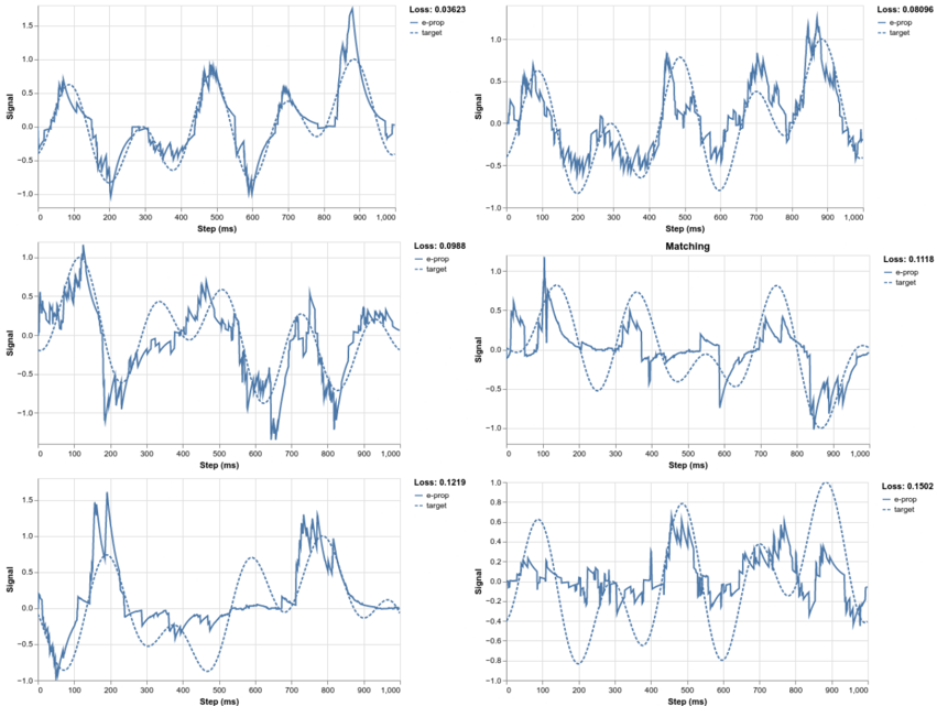
The image contains six line graphs arranged in two columns and three rows, comparing two data series labeled "e-prop" (solid blue line) and "target" (dashed blue line). Each graph visualizes signal values over time steps (0–1000 ms) and includes a loss metric in the top-right corner. The y-axis ranges from -1.5 to 1.5, while the x-axis spans 0–1000 ms. All graphs share identical axis labels and legend placement but differ in loss values and line behavior.
### Components/Axes
- **X-axis**: "Step (ms)" with ticks at 0, 100, 200, ..., 1000.
- **Y-axis**: "Signal" with ticks at -1.5, -1.0, -0.5, 0.0, 0.5, 1.0, 1.5.
- **Legend**: Located in the top-right corner of each graph, with:
- Solid blue line: "e-prop"
- Dashed blue line: "target"
- **Loss Values**: Displayed in the top-right corner of each graph (e.g., "Loss: 0.03623").
### Detailed Analysis
1. **Top-Left Graph (Loss: 0.03623)**
- **Trend**: The "e-prop" line closely mirrors the "target" line, with minor deviations. Both lines exhibit sharp peaks (~1.2) and troughs (~-1.0) around steps 100–200 and 500–600 ms.
- **Key Points**:
- Peak at ~100 ms: e-prop ≈ 1.2, target ≈ 1.1.
- Trough at ~200 ms: e-prop ≈ -1.0, target ≈ -0.9.
- Final step (1000 ms): Both lines converge near 0.1.
2. **Top-Right Graph (Loss: 0.08096)**
- **Trend**: "e-prop" deviates significantly from "target," particularly during oscillations. Peaks and troughs are less synchronized.
- **Key Points**:
- Peak at ~300 ms: e-prop ≈ 0.8, target ≈ 0.6.
- Trough at ~700 ms: e-prop ≈ -0.7, target ≈ -0.5.
- Final step: e-prop ≈ 0.3, target ≈ 0.1.
3. **Middle-Left Graph (Loss: 0.0988)**
- **Trend**: "e-prop" lags behind "target" during rapid transitions. Peaks are delayed by ~50 ms.
- **Key Points**:
- Peak at ~400 ms: e-prop ≈ 0.7, target ≈ 0.9.
- Trough at ~800 ms: e-prop ≈ -0.6, target ≈ -0.8.
4. **Middle-Right Graph (Loss: 0.1118)**
- **Trend**: "e-prop" exhibits erratic behavior, with overshoots and undershoots relative to "target."
- **Key Points**:
- Peak at ~600 ms: e-prop ≈ 1.1, target ≈ 0.7.
- Trough at ~900 ms: e-prop ≈ -0.9, target ≈ -0.5.
5. **Bottom-Left Graph (Loss: 0.1219)**
- **Trend**: "e-prop" underperforms, with flattened peaks and delayed responses.
- **Key Points**:
- Peak at ~200 ms: e-prop ≈ 0.5, target ≈ 0.8.
- Trough at ~700 ms: e-prop ≈ -0.4, target ≈ -0.7.
6. **Bottom-Right Graph (Loss: 0.1502)**
- **Trend**: "e-prop" shows the largest divergence, with irregular oscillations and poor synchronization.
- **Key Points**:
- Peak at ~500 ms: e-prop ≈ 0.9, target ≈ 0.6.
- Trough at ~900 ms: e-prop ≈ -1.0, target ≈ -0.8.
### Key Observations
- **Loss Correlation**: Lower loss values (e.g., 0.03623) correspond to tighter alignment between "e-prop" and "target." Higher losses (e.g., 0.1502) indicate greater divergence.
- **Temporal Patterns**: Peaks and troughs in "e-prop" often lag or overshoot "target," especially in high-loss graphs.
- **Signal Range**: Both lines consistently stay within -1.5 to 1.5, but "e-prop" exhibits more extreme fluctuations in high-loss cases.
### Interpretation
The data suggests that "e-prop" performance varies across trials, with lower loss values indicating better model accuracy in replicating the "target" signal. The visual trends reveal that discrepancies arise primarily during rapid transitions (e.g., peaks/troughs), where "e-prop" either delays or overcompensates. The loss metric quantifies these deviations, providing a numerical benchmark for model refinement. Notably, the highest-loss graph (0.1502) demonstrates systemic instability, suggesting potential issues with model training or data preprocessing in that trial.