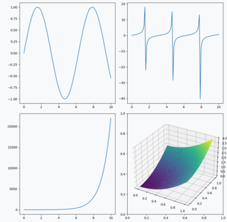
\n ## Charts: Four Mathematical Function Plots ### Overview The image presents four separate 2D and 3D plots of mathematical functions. Each plot displays a different function, with varying scales and characteristics. There are no explicit labels or legends provided within the image itself. The plots are arranged in a 2x2 grid. ### Components/Axes * **Top-Left Plot:** X-axis ranges from approximately 0 to 10, Y-axis ranges from approximately -3 to 2. * **Top-Right Plot:** X-axis ranges from approximately 0 to 5, Y-axis ranges from approximately -3 to 2. * **Bottom-Left Plot:** X-axis ranges from approximately 0 to 10, Y-axis ranges from approximately 0 to 20000. * **Bottom-Right Plot:** X and Y axes both range from approximately 0 to 1. Z-axis ranges from approximately 0 to 15. This is a 3D surface plot. ### Detailed Analysis or Content Details **Top-Left Plot:** The plot shows a periodic function resembling a cosine wave. The function completes approximately one and a half cycles within the displayed range. * At x = 0, y ≈ 1.5 * At x = 2.5, y ≈ -2.5 (minimum) * At x = 5, y ≈ 1.5 * At x = 7.5, y ≈ -2.5 (minimum) * At x = 10, y ≈ 1.5 **Top-Right Plot:** This plot displays a function with vertical asymptotes. It appears to be a periodic function with singularities. * There are vertical asymptotes near x = 1, x = 3, and x = 5. * Between asymptotes, the function oscillates rapidly between positive and negative values. * At x = 0.5, y ≈ -1.5 * At x = 1.5, y ≈ 1.5 * At x = 2.5, y ≈ -1.5 * At x = 4.5, y ≈ 1.5 **Bottom-Left Plot:** This plot shows a rapidly increasing function, likely exponential or polynomial of high degree. * At x = 0, y ≈ 1 * At x = 2, y ≈ 100 * At x = 4, y ≈ 1000 * At x = 6, y ≈ 5000 * At x = 8, y ≈ 15000 * At x = 10, y ≈ 20000 **Bottom-Right Plot:** This is a 3D surface plot. The color gradient indicates the value of the function. * The surface is curved, rising from left to right and from bottom to top. * The lowest values (dark purple) are near x = 0 and y = 0. * The highest values (yellow/green) are near x = 1 and y = 1. * The function appears to be increasing in both x and y directions. ### Key Observations * The top-left plot demonstrates a smooth, periodic behavior. * The top-right plot exhibits a more complex, discontinuous behavior with asymptotes. * The bottom-left plot shows exponential growth. * The bottom-right plot visualizes a function of two variables, showing a curved surface. * There is no common scale or units indicated for any of the axes. ### Interpretation The image presents a visual comparison of different mathematical functions. The functions chosen represent a range of behaviors, from simple periodic oscillations to exponential growth and more complex, discontinuous patterns. The 3D plot adds a dimension of complexity, illustrating a function of two variables. The lack of labels makes it difficult to determine the specific functions being plotted, but the visual characteristics provide clues about their nature. The plots could be used to illustrate concepts in calculus, analysis, or numerical methods. The exponential growth in the bottom-left plot could represent population growth, compound interest, or other phenomena that exhibit similar behavior. The asymptotes in the top-right plot could represent physical limitations or singularities in a system. The 3D plot could represent a surface in physics, engineering, or computer graphics.