## [Chart Type]: Two Subplots (Scatter Plots with Trend Lines and ACF vs Lag)
### Overview
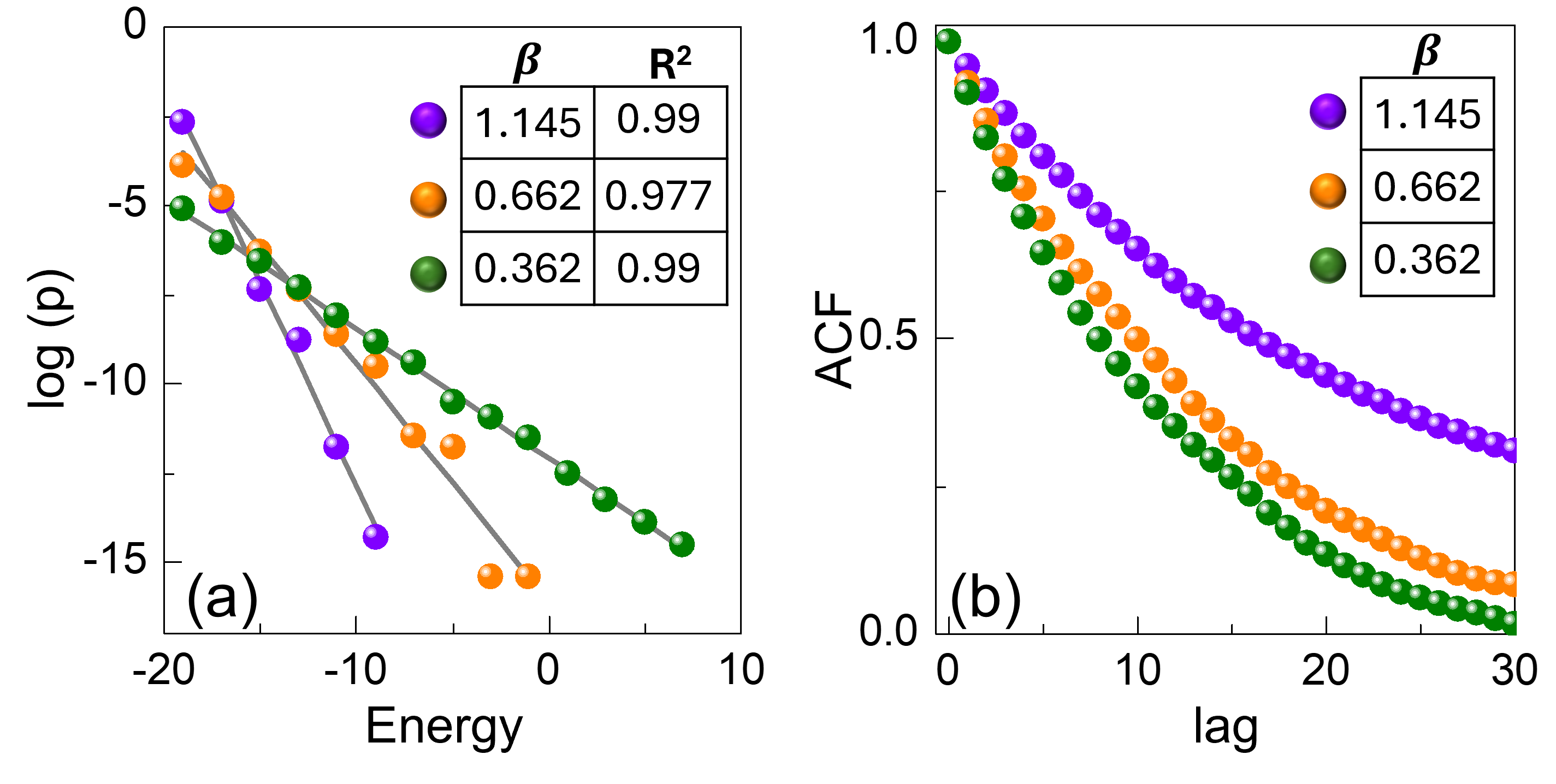
The image contains two side-by-side subplots (labeled (a) and (b)) analyzing relationships involving a parameter \( \boldsymbol{\beta} \). Subplot (a) shows \( \log(p) \) vs. Energy with linear trend lines, while subplot (b) shows Autocorrelation Function (ACF) vs. lag. Both use three color-coded data series (purple, orange, green) corresponding to \( \beta = 1.145 \), \( 0.662 \), and \( 0.362 \), respectively.
### Components/Axes
#### Subplot (a) (Left):
- **X-axis**: Label = "Energy", Range = \([-20, 10]\), Ticks = \(-20, -10, 0, 10\).
- **Y-axis**: Label = "log(p)", Range = \([-15, 0]\), Ticks = \(-15, -10, -5, 0\).
- **Legend**: Top-right, with three entries:
- Purple: \( \beta = 1.145 \), \( R^2 = 0.99 \)
- Orange: \( \beta = 0.662 \), \( R^2 = 0.977 \)
- Green: \( \beta = 0.362 \), \( R^2 = 0.99 \)
- **Data Series**: Scatter points with linear trend lines (gray) for each \( \beta \).
#### Subplot (b) (Right):
- **X-axis**: Label = "lag", Range = \([0, 30]\), Ticks = \(0, 10, 20, 30\).
- **Y-axis**: Label = "ACF", Range = \([0.0, 1.0]\), Ticks = \(0.0, 0.5, 1.0\).
- **Legend**: Top-right, with three entries (same \( \beta \) values as (a)):
- Purple: \( \beta = 1.145 \)
- Orange: \( \beta = 0.662 \)
- Green: \( \beta = 0.362 \)
- **Data Series**: Scatter points (no trend lines) for each \( \beta \).
### Detailed Analysis
#### Subplot (a) (log(p) vs. Energy):
- **Trend Verification**: All three series show a **decreasing trend** (log(p) decreases as Energy increases).
- Purple (\( \beta = 1.145 \)): Steepest slope (e.g., at Energy = \(-20\), log(p) ≈ \(-5\); at Energy = \(-10\), log(p) ≈ \(-15\)).
- Orange (\( \beta = 0.662 \)): Moderate slope (e.g., at Energy = \(-20\), log(p) ≈ \(-5\); at Energy = \(-10\), log(p) ≈ \(-12\)).
- Green (\( \beta = 0.362 \)): Shallowest slope (e.g., at Energy = \(-20\), log(p) ≈ \(-5\); at Energy = \(-10\), log(p) ≈ \(-10\)).
- **R² Values**: Purple and green have \( R^2 = 0.99 \) (excellent linear fit); orange has \( R^2 = 0.977 \) (good fit).
#### Subplot (b) (ACF vs. lag):
- **Trend Verification**: All three series show a **decreasing trend** (ACF decreases as lag increases).
- Purple (\( \beta = 1.145 \)): Slowest decay (e.g., at lag = 0, ACF ≈ \(1.0\); at lag = 30, ACF ≈ \(0.3\)).
- Orange (\( \beta = 0.662 \)): Moderate decay (e.g., at lag = 0, ACF ≈ \(1.0\); at lag = 30, ACF ≈ \(0.2\)).
- Green (\( \beta = 0.362 \)): Fastest decay (e.g., at lag = 0, ACF ≈ \(1.0\); at lag = 30, ACF ≈ \(0.1\)).
### Key Observations
- In (a), \( \log(p) \) decreases with Energy for all \( \beta \), with steeper slopes for higher \( \beta \).
- In (b), ACF decays with lag for all \( \beta \), with slower decay for higher \( \beta \).
- High \( R^2 \) values in (a) confirm strong linear relationships between \( \log(p) \) and Energy.
### Interpretation
- **Subplot (a)**: The linear relationship between \( \log(p) \) and Energy (high \( R^2 \)) suggests a consistent statistical/physical model. Higher \( \beta \) accelerates the decrease of \( \log(p) \) with Energy, implying \( \beta \) modulates the energy-probability relationship.
- **Subplot (b)**: ACF decay rate inversely correlates with \( \beta \): higher \( \beta \) means longer-range correlations (ACF stays higher for longer lags), while lower \( \beta \) means shorter-range correlations. This suggests \( \beta \) controls the temporal/spatial correlation structure.
- **Overall**: The two plots link \( \beta \) to both the energy-probability relationship (a) and the autocorrelation decay (b), indicating \( \beta \) is a key parameter governing the system’s statistical behavior.
(No non-English text is present; all labels and text are in English.)