## Scatter Plots: Relationship Between Energy, ACF, and β Parameter
### Overview
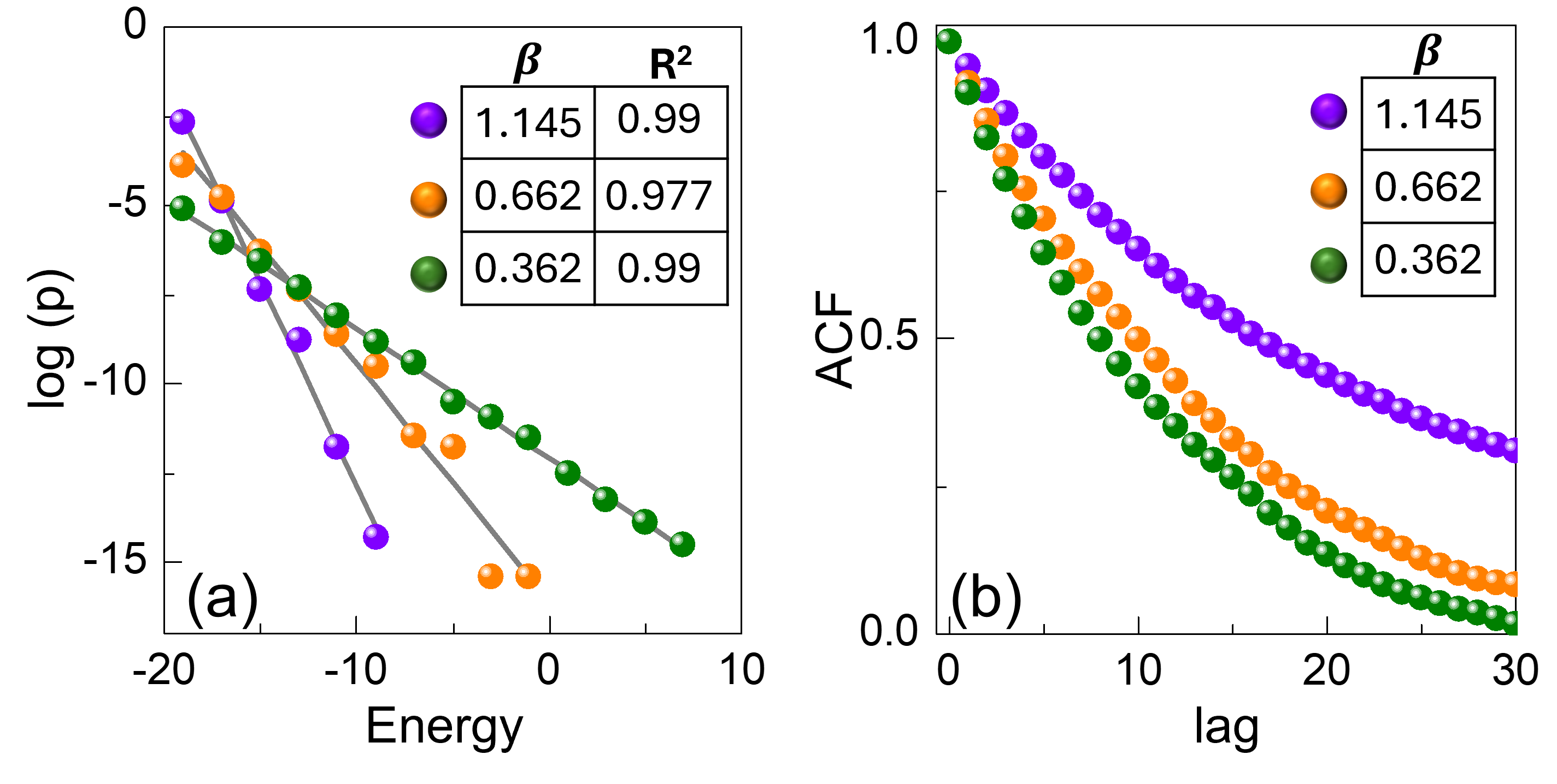
The image contains two scatter plots labeled (a) and (b), analyzing relationships between variables with three distinct β (beta) parameter values. Both plots use color-coded data points (purple, orange, green) to represent different β values, with high R² values indicating strong linear or autocorrelation patterns.
---
### Components/Axes
#### Plot (a)
- **X-axis**: Energy (ranging from -20 to 10)
- **Y-axis**: log(p) (ranging from -15 to 0)
- **Legend**:
- Purple: β = 1.145 (R² = 0.99)
- Orange: β = 0.662 (R² = 0.977)
- Green: β = 0.362 (R² = 0.99)
- **Trend**: All three lines show a steep downward slope, with purple (β=1.145) being the steepest.
#### Plot (b)
- **X-axis**: lag (ranging from 0 to 30)
- **Y-axis**: ACF (Autocorrelation Function, ranging from 0 to 1)
- **Legend**:
- Purple: β = 1.145
- Orange: β = 0.662
- Green: β = 0.362
- **Trend**: All three lines show a gradual decline, with purple (β=1.145) starting highest and green (β=0.362) ending lowest.
---
### Detailed Analysis
#### Plot (a)
- **Data Points**:
- Purple (β=1.145): Points tightly clustered along a steep linear regression line (R²=0.99).
- Orange (β=0.662): Slightly less steep slope (R²=0.977), with minor deviations.
- Green (β=0.362): Flattest slope (R²=0.99), indicating near-perfect linear fit despite lower β.
- **Spatial Grounding**: Legend positioned in the top-right corner of the plot.
#### Plot (b)
- **Data Points**:
- Purple (β=1.145): Highest initial ACF values, decaying slowly with lag.
- Orange (β=0.662): Intermediate decay rate.
- Green (β=0.362): Fastest decay, reaching near-zero ACF at lower lags.
- **Spatial Grounding**: Legend positioned in the top-right corner of the plot.
---
### Key Observations
1. **Plot (a)**:
- All β values show strong linear relationships (R² ≥ 0.977).
- Higher β values correspond to steeper slopes, suggesting a direct relationship between β and the rate of change in log(p) with energy.
- Green (β=0.362) has the flattest slope despite the highest R², indicating minimal energy dependence.
2. **Plot (b)**:
- ACF decays with increasing lag for all β values, consistent with diminishing autocorrelation over time/intervals.
- Higher β values (e.g., purple) retain stronger initial autocorrelation, while lower β values (green) exhibit rapid decay.
---
### Interpretation
- **Plot (a)** suggests that the parameter β modulates the sensitivity of log(p) to energy changes. Higher β values (e.g., 1.145) imply a stronger dependency, while lower β values (e.g., 0.362) indicate near-independence. The near-perfect R² values suggest the linear models are highly reliable.
- **Plot (b)** reveals that β also influences the autocorrelation structure. Higher β values maintain stronger correlations over longer lags, potentially indicating persistent dependencies in the system. The decay patterns align with typical time-series behavior, where correlations weaken as temporal or spatial separation increases.
- **Cross-Plot Insight**: The consistent β values across both plots imply a unified parameter governing both energy-response dynamics (Plot a) and temporal autocorrelation (Plot b). This could reflect a physical or statistical property (e.g., damping, memory) in the underlying system.