## Multiple Line Charts: Accuracy vs. Parameter C for Different K and r Values
### Overview
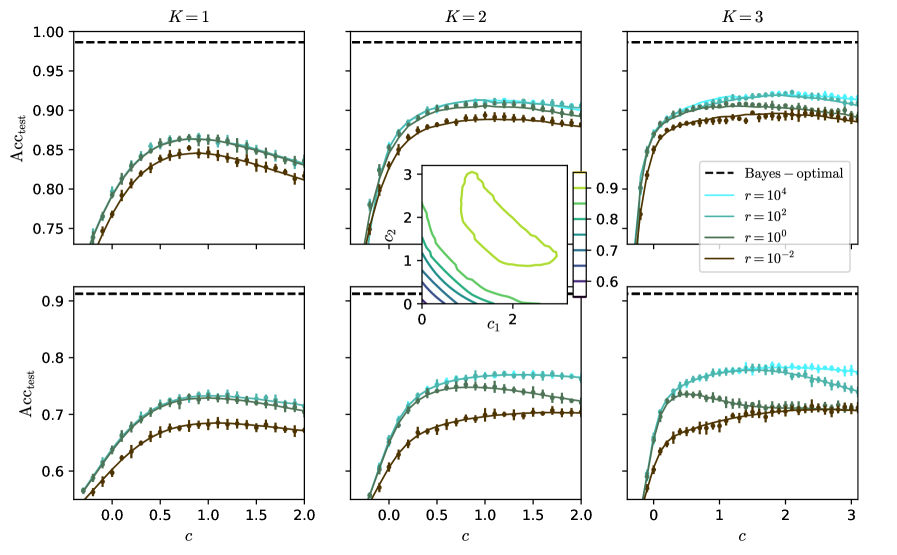
The image contains six line charts arranged in a 2x3 grid. Each chart plots the test accuracy (Acc_test) against a parameter 'c' for different values of 'K' (K=1, K=2, K=3). Within each chart, multiple lines represent different values of 'r' (r=10^4, r=10^2, r=10^0, r=10^-2). A dashed horizontal line indicates the Bayes-optimal accuracy. An inset contour plot in the K=2 chart shows the relationship between parameters c1 and c2.
### Components/Axes
* **Titles:** Each of the six charts has a title indicating the value of K: "K=1", "K=2", "K=3" (repeated in the top and bottom rows).
* **Y-axis:** The y-axis is labeled "Acc_test" and ranges from approximately 0.75 to 1.00 in the top row and from approximately 0.6 to 0.9 in the bottom row.
* **X-axis:** The x-axis is labeled "c". The range varies depending on the column: approximately 0 to 2 for K=1, 0 to 2 for K=2, and 0 to 3 for K=3.
* **Legend:** Located to the right of the K=2 chart, the legend identifies the lines:
* Black dashed line: "Bayes - optimal"
* Light blue line: "r = 10^4"
* Darker blue/green line: "r = 10^2"
* Gray/Green line: "r = 10^0"
* Brown line: "r = 10^-2"
* **Inset Contour Plot (K=2 chart):**
* X-axis: "c1" ranging from 0 to approximately 2.
* Y-axis: "c2" ranging from 0 to approximately 3.
* Contours: Represent accuracy values from 0.6 to 0.9, with increasing accuracy as the color shifts from blue to yellow/green.
### Detailed Analysis
**Chart Row 1 (Top Row):**
* **K = 1:**
* Bayes-optimal: Approximately 0.99
* r = 10^4 (light blue): Starts at approximately 0.73, rises to a peak around 0.86 at c=0.75, then decreases to approximately 0.82 at c=2.0.
* r = 10^2 (darker blue/green): Starts at approximately 0.73, rises to a peak around 0.85 at c=0.75, then decreases to approximately 0.81 at c=2.0.
* r = 10^0 (gray/green): Not present in this chart.
* r = 10^-2 (brown): Starts at approximately 0.73, rises to a peak around 0.84 at c=0.75, then decreases to approximately 0.81 at c=2.0.
* **K = 2:**
* Bayes-optimal: Approximately 0.99
* r = 10^4 (light blue): Starts at approximately 0.73, rises to a peak around 0.92 at c=1.25, then decreases to approximately 0.90 at c=2.0.
* r = 10^2 (darker blue/green): Starts at approximately 0.73, rises to a peak around 0.90 at c=1.25, then decreases to approximately 0.88 at c=2.0.
* r = 10^0 (gray/green): Not present in this chart.
* r = 10^-2 (brown): Starts at approximately 0.73, rises to a peak around 0.89 at c=1.25, then decreases to approximately 0.87 at c=2.0.
* **K = 3:**
* Bayes-optimal: Approximately 0.99
* r = 10^4 (light blue): Starts at approximately 0.73, rises to a peak around 0.93 at c=1.5, then decreases to approximately 0.91 at c=3.0.
* r = 10^2 (darker blue/green): Starts at approximately 0.73, rises to a peak around 0.90 at c=1.5, then decreases to approximately 0.89 at c=3.0.
* r = 10^0 (gray/green): Not present in this chart.
* r = 10^-2 (brown): Starts at approximately 0.73, rises to a peak around 0.89 at c=1.5, then decreases to approximately 0.87 at c=3.0.
**Chart Row 2 (Bottom Row):**
* **K = 1:**
* Bayes-optimal: Approximately 0.90
* r = 10^4 (light blue): Starts at approximately 0.55, rises to a peak around 0.73 at c=1.0, then remains relatively constant.
* r = 10^2 (darker blue/green): Not present in this chart.
* r = 10^0 (gray/green): Not present in this chart.
* r = 10^-2 (brown): Starts at approximately 0.55, rises to a peak around 0.68 at c=0.75, then remains relatively constant.
* **K = 2:**
* Bayes-optimal: Approximately 0.90
* r = 10^4 (light blue): Starts at approximately 0.55, rises to a peak around 0.77 at c=1.25, then remains relatively constant.
* r = 10^2 (darker blue/green): Not present in this chart.
* r = 10^0 (gray/green): Not present in this chart.
* r = 10^-2 (brown): Starts at approximately 0.55, rises to a peak around 0.73 at c=1.0, then remains relatively constant.
* **K = 3:**
* Bayes-optimal: Approximately 0.90
* r = 10^4 (light blue): Starts at approximately 0.55, rises to a peak around 0.78 at c=1.5, then remains relatively constant.
* r = 10^2 (darker blue/green): Starts at approximately 0.55, rises to a peak around 0.73 at c=1.0, then remains relatively constant.
* r = 10^0 (gray/green): Not present in this chart.
* r = 10^-2 (brown): Starts at approximately 0.55, rises to a peak around 0.70 at c=0.75, then remains relatively constant.
### Key Observations
* The Bayes-optimal accuracy is higher in the top row (approximately 0.99) compared to the bottom row (approximately 0.90).
* In the top row, the accuracy generally increases with increasing 'K' for a given 'r'.
* In the top row, the accuracy generally decreases with decreasing 'r' for a given 'K'.
* In the bottom row, the accuracy generally increases with increasing 'K' for a given 'r'.
* In the bottom row, the accuracy generally decreases with decreasing 'r' for a given 'K'.
* The inset contour plot in the K=2 chart shows a positive correlation between c1 and c2 for achieving higher accuracy.
* The lines in the bottom row appear to plateau after reaching their peak accuracy.
### Interpretation
The charts illustrate the impact of parameters 'K', 'r', and 'c' on the test accuracy of a model. The top row likely represents a different experimental setup or dataset compared to the bottom row, as evidenced by the higher Bayes-optimal accuracy. The value of 'K' seems to positively influence accuracy, suggesting that increasing 'K' improves model performance up to a point. The parameter 'r' also plays a significant role, with higher values generally leading to better accuracy. The parameter 'c' appears to have an optimal value for each combination of 'K' and 'r', as the accuracy curves exhibit a peak. The contour plot suggests that specific combinations of c1 and c2 are crucial for achieving high accuracy when K=2. The plateauing of accuracy in the bottom row might indicate a saturation effect, where further increases in 'c' do not lead to significant improvements in performance.