TECHNICAL ASSET FINGERPRINT
82d7e00c0acaa8756e6c6bcc
Click to view fullscreen
Press ESC or click to close
FOUND IN PAPERS
EXPERT: gemma-3-27b-it-free VERSION 1
RUNTIME: google-free/gemma-3-27b-it
INTEL_VERIFIED
## Chart: Accuracy vs. Regularization Parameter
### Overview
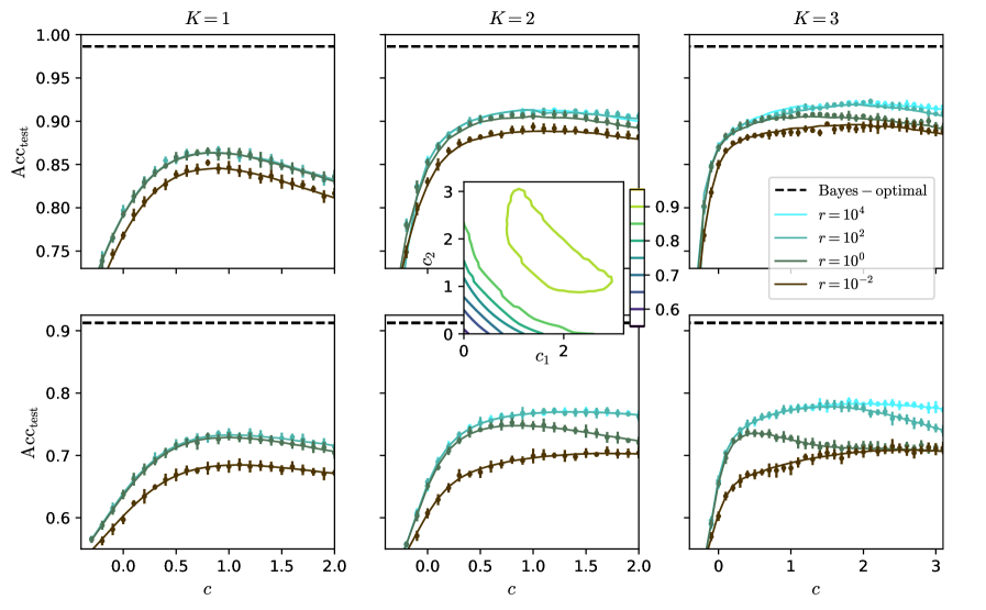
The image presents a series of six line plots, arranged in a 2x3 grid, illustrating the relationship between accuracy and a regularization parameter 'c' for different values of 'K' (1, 2, and 3) and 'r' (10<sup>-2</sup>, 10<sup>0</sup>, 10<sup>2</sup>, 10<sup>4</sup>). The top row displays accuracy on the test set (Acc<sub>test</sub>), while the bottom row displays accuracy on the cost set (Acc<sub>cost</sub>). A contour plot is included in the center column, showing the relationship between c<sub>1</sub> and c<sub>2</sub>.
### Components/Axes
* **X-axis (all plots except contour):** 'c', ranging from approximately 0.0 to 3.0.
* **Y-axis (top row):** Acc<sub>test</sub>, ranging from approximately 0.7 to 1.0.
* **Y-axis (bottom row):** Acc<sub>cost</sub>, ranging from approximately 0.6 to 0.9.
* **Contour Plot X-axis:** c<sub>1</sub>, ranging from approximately 0.0 to 2.0.
* **Contour Plot Y-axis:** c<sub>2</sub>, ranging from approximately 0.0 to 3.0.
* **Legend (top-right):**
* `-- Bayes – optimal` (dashed black line)
* `r = 10^4` (solid dark grey line)
* `r = 10^2` (solid medium grey line)
* `r = 10^0` (solid light grey line)
* `r = 10^-2` (solid teal line)
* **Titles (top of each plot):** K = 1, K = 2, K = 3.
* **Vertical dashed lines:** Present in each plot, positioned at approximately c = 0.5, 1.5, and 2.5.
### Detailed Analysis or Content Details
**K = 1 (Left Column)**
* **Acc<sub>test</sub>:** The Bayes-optimal line (dashed black) is flat at approximately 0.96. The r = 10<sup>4</sup> line (dark grey) starts at approximately 0.80 and increases rapidly to approximately 0.95 by c = 1.5, then plateaus. The r = 10<sup>2</sup> line (medium grey) starts at approximately 0.78 and increases more gradually, reaching approximately 0.92 by c = 2.0. The r = 10<sup>0</sup> line (light grey) starts at approximately 0.75 and increases slowly, reaching approximately 0.88 by c = 2.0. The r = 10<sup>-2</sup> line (teal) starts at approximately 0.72 and increases steadily, reaching approximately 0.85 by c = 2.0.
* **Acc<sub>cost</sub>:** The Bayes-optimal line (dashed black) is flat at approximately 0.90. The r = 10<sup>4</sup> line (dark grey) starts at approximately 0.62 and increases rapidly to approximately 0.85 by c = 1.5, then plateaus. The r = 10<sup>2</sup> line (medium grey) starts at approximately 0.60 and increases more gradually, reaching approximately 0.80 by c = 2.0. The r = 10<sup>0</sup> line (light grey) starts at approximately 0.58 and increases slowly, reaching approximately 0.75 by c = 2.0. The r = 10<sup>-2</sup> line (teal) starts at approximately 0.56 and increases steadily, reaching approximately 0.70 by c = 2.0.
**K = 2 (Center Column)**
* **Acc<sub>test</sub>:** The Bayes-optimal line (dashed black) is flat at approximately 0.96. The r = 10<sup>4</sup> line (dark grey) starts at approximately 0.85 and increases rapidly to approximately 0.96 by c = 1.0, then plateaus. The r = 10<sup>2</sup> line (medium grey) starts at approximately 0.82 and increases more gradually, reaching approximately 0.94 by c = 2.0. The r = 10<sup>0</sup> line (light grey) starts at approximately 0.78 and increases slowly, reaching approximately 0.90 by c = 2.0. The r = 10<sup>-2</sup> line (teal) starts at approximately 0.75 and increases steadily, reaching approximately 0.87 by c = 2.0.
* **Acc<sub>cost</sub>:** The Bayes-optimal line (dashed black) is flat at approximately 0.90. The r = 10<sup>4</sup> line (dark grey) starts at approximately 0.68 and increases rapidly to approximately 0.88 by c = 1.0, then plateaus. The r = 10<sup>2</sup> line (medium grey) starts at approximately 0.65 and increases more gradually, reaching approximately 0.80 by c = 2.0. The r = 10<sup>0</sup> line (light grey) starts at approximately 0.62 and increases slowly, reaching approximately 0.75 by c = 2.0. The r = 10<sup>-2</sup> line (teal) starts at approximately 0.60 and increases steadily, reaching approximately 0.70 by c = 2.0.
* **Contour Plot:** The contour plot shows level curves representing different values. The yellow contour (approximately 0.9) is elongated and curves from the bottom-left to the top-right. The teal contour (approximately 0.7) is more circular and centered around c<sub>1</sub> = 0.5 and c<sub>2</sub> = 1.5.
**K = 3 (Right Column)**
* **Acc<sub>test</sub>:** The Bayes-optimal line (dashed black) is flat at approximately 0.96. The r = 10<sup>4</sup> line (dark grey) starts at approximately 0.90 and increases rapidly to approximately 0.98 by c = 1.0, then plateaus. The r = 10<sup>2</sup> line (medium grey) starts at approximately 0.87 and increases more gradually, reaching approximately 0.96 by c = 2.0. The r = 10<sup>0</sup> line (light grey) starts at approximately 0.83 and increases slowly, reaching approximately 0.92 by c = 2.0. The r = 10<sup>-2</sup> line (teal) starts at approximately 0.80 and increases steadily, reaching approximately 0.89 by c = 2.0.
* **Acc<sub>cost</sub>:** The Bayes-optimal line (dashed black) is flat at approximately 0.90. The r = 10<sup>4</sup> line (dark grey) starts at approximately 0.75 and increases rapidly to approximately 0.90 by c = 1.0, then plateaus. The r = 10<sup>2</sup> line (medium grey) starts at approximately 0.70 and increases more gradually, reaching approximately 0.85 by c = 2.0. The r = 10<sup>0</sup> line (light grey) starts at approximately 0.65 and increases slowly, reaching approximately 0.80 by c = 2.0. The r = 10<sup>-2</sup> line (teal) starts at approximately 0.60 and increases steadily, reaching approximately 0.75 by c = 2.0.
### Key Observations
* As 'K' increases, the accuracy generally increases for a given 'c' and 'r'.
* Larger values of 'r' (e.g., 10<sup>4</sup>) lead to faster convergence to higher accuracy, but may overfit.
* Smaller values of 'r' (e.g., 10<sup>-2</sup>) lead to slower convergence and lower accuracy, but may generalize better.
* The Bayes-optimal line represents an upper bound on achievable accuracy.
* The contour plot suggests an optimal region for c<sub>1</sub> and c<sub>2</sub> that maximizes accuracy.
### Interpretation
The plots demonstrate the trade-off between bias and variance in a model with a regularization parameter 'c'. Increasing 'c' reduces variance (overfitting) but may increase bias (underfitting). The optimal value of 'c' depends on the complexity of the model ('K') and the strength of the regularization ('r'). The contour plot provides a visual representation of this trade-off in a two-dimensional parameter space. The dashed black line representing the Bayes-optimal solution serves as a benchmark, indicating the maximum achievable accuracy given the data and model. The different lines representing different values of 'r' show how the regularization strength affects the model's performance. The vertical dashed lines may indicate points of interest for further analysis, potentially representing critical values of 'c' where the model's behavior changes significantly. The difference between Acc<sub>test</sub> and Acc<sub>cost</sub> suggests a potential discrepancy between the model's performance on the training and testing data, which could be indicative of overfitting or underfitting.
DECODING INTELLIGENCE...