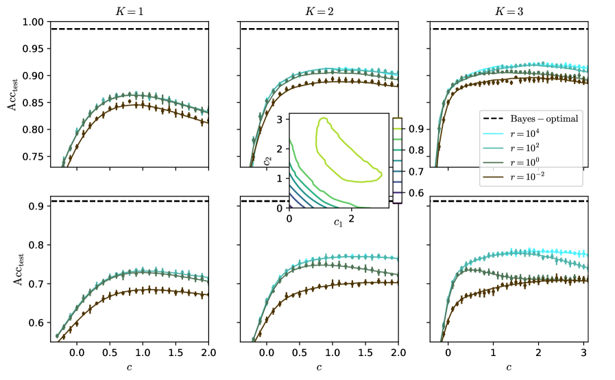
## Line Plots with Error Bars: Test Accuracy vs. Parameter `c` for Different `r` and `K` Values ### Overview The image displays a 2x3 grid of line plots showing the relationship between a parameter `c` (x-axis) and test accuracy (`Acc_test`, y-axis). Each column corresponds to a different value of `K` (1, 2, 3). Each plot contains multiple data series representing different values of a parameter `r`. A dashed horizontal line indicates the "Bayes-optimal" accuracy. An inset contour plot is embedded within the middle-top plot (`K=2`). ### Components/Axes * **Grid Structure:** Two rows, three columns. * **Column Titles (Top of each column):** `K = 1`, `K = 2`, `K = 3`. * **Y-axis Label (Left side of both rows):** `Acc_test` (Test Accuracy). * **X-axis Label (Bottom of both rows):** `c`. * **Legend (Located in the top-right plot, `K=3`):** * `--- Bayes-optimal` (Black dashed line) * `r = 10^4` (Cyan line with '+' markers) * `r = 10^2` (Teal line with '+' markers) * `r = 10^0` (Dark green line with '+' markers) * `r = 10^{-2}` (Brown line with '+' markers) * **Inset Plot (Within the `K=2`, top row plot):** * **X-axis Label:** `c1` * **Y-axis Label:** `c2` * **Color Bar (Right side of inset):** Values ranging from approximately 0.6 to 0.9, indicating a third dimension (likely accuracy). * **Content:** Contour lines showing regions of constant value in the (`c1`, `c2`) parameter space. ### Detailed Analysis **General Trend Across All Plots:** For all series, `Acc_test` initially increases as `c` increases from 0, reaches a peak, and then gradually decreases or plateaus as `c` continues to increase. The Bayes-optimal line is a constant horizontal benchmark. **Top Row (First set of experiments):** * **`K=1` (Top-Left):** * **Bayes-optimal:** ~0.985. * **Trend:** All curves peak around `c ≈ 0.8-1.0`. * **Data Points (Approximate Peak Accuracies):** * `r=10^4` (Cyan): Peaks at ~0.87. * `r=10^2` (Teal): Peaks at ~0.86. * `r=10^0` (Green): Peaks at ~0.85. * `r=10^{-2}` (Brown): Peaks at ~0.84. * **Order:** Higher `r` yields higher accuracy. The gap between `r=10^4` and `r=10^2` is small. * **`K=2` (Top-Middle):** * **Bayes-optimal:** ~0.985. * **Trend:** Curves rise sharply and plateau. Peak is broader, around `c ≈ 0.8-1.5`. * **Data Points (Approximate Plateau Accuracies):** * `r=10^4` (Cyan): Plateaus at ~0.91. * `r=10^2` (Teal): Plateaus at ~0.90. * `r=10^0` (Green): Plateaus at ~0.89. * `r=10^{-2}` (Brown): Plateaus at ~0.88. * **Inset Plot:** Shows a contour map in (`c1`, `c2`) space. The contours form a diagonal, elongated valley/ridge structure, suggesting a correlation or trade-off between `c1` and `c2` for achieving a given performance level. The color bar indicates performance ranges from ~0.6 to >0.9. * **`K=3` (Top-Right):** * **Bayes-optimal:** ~0.985. * **Trend:** Similar to `K=2`, sharp rise to a plateau. * **Data Points (Approximate Plateau Accuracies):** * `r=10^4` (Cyan): Plateaus at ~0.92. * `r=10^2` (Teal): Plateaus at ~0.91. * `r=10^0` (Green): Plateaus at ~0.90. * `r=10^{-2}` (Brown): Plateaus at ~0.89. * **Note:** The x-axis extends to `c=3`, showing the plateau continues. **Bottom Row (Second set of experiments):** * **`K=1` (Bottom-Left):** * **Bayes-optimal:** ~0.91. * **Trend:** Peaks around `c ≈ 0.8-1.0`. * **Data Points (Approximate Peak Accuracies):** * `r=10^4` (Cyan): Peaks at ~0.74. * `r=10^2` (Teal): Peaks at ~0.73. * `r=10^0` (Green): Peaks at ~0.69. * `r=10^{-2}` (Brown): Peaks at ~0.68. * **Note:** Overall accuracy is lower than the top row. The gap between `r=10^2` and `r=10^0` is more pronounced. * **`K=2` (Bottom-Middle):** * **Bayes-optimal:** ~0.91. * **Trend:** Rises to a plateau around `c ≈ 1.0-1.5`. * **Data Points (Approximate Plateau Accuracies):** * `r=10^4` (Cyan): Plateaus at ~0.77. * `r=10^2` (Teal): Plateaus at ~0.76. * `r=10^0` (Green): Plateaus at ~0.71. * `r=10^{-2}` (Brown): Plateaus at ~0.70. * **`K=3` (Bottom-Right):** * **Bayes-optimal:** ~0.91. * **Trend:** Rises to a plateau around `c ≈ 1.5-2.0`. * **Data Points (Approximate Plateau Accuracies):** * `r=10^4` (Cyan): Plateaus at ~0.78. * `r=10^2` (Teal): Plateaus at ~0.77. * `r=10^0` (Green): Plateaus at ~0.72. * `r=10^{-2}` (Brown): Plateaus at ~0.71. ### Key Observations 1. **Effect of `r`:** In every subplot, higher values of `r` (10^4, cyan) consistently yield higher test accuracy than lower values (10^{-2}, brown). The performance gap between `r=10^4` and `r=10^2` is generally smaller than the gap between `r=10^0` and `r=10^{-2}`. 2. **Effect of `K`:** Moving from left to right (`K=1` to `K=3`), the peak/plateau accuracy increases within each row. The shape of the curve also changes from a distinct peak (`K=1`) to a broader plateau (`K=2,3`). 3. **Effect of Row (Experimental Condition):** The top row achieves significantly higher absolute accuracy (peaks ~0.84-0.92) compared to the bottom row (peaks ~0.68-0.78). The Bayes-optimal benchmark is also higher in the top row (~0.985 vs ~0.91). 4. **Parameter `c`:** There is an optimal range for `c` (typically 0.5 to 2.0) that maximizes accuracy. Setting `c` too low or too high degrades performance. 5. **Inset Plot:** The contour plot for `K=2` suggests the existence of a two-dimensional parameter space (`c1`, `c2`) where performance is optimized along a specific manifold or valley. ### Interpretation This figure likely comes from a machine learning or statistical modeling paper investigating the performance of an algorithm under different hyperparameter settings (`K`, `r`, `c`). The two rows probably represent two different datasets or problem difficulties (the top row being "easier," given the higher Bayes-optimal and achieved accuracies). * **`K`** likely represents model complexity or capacity (e.g., number of components, layers, or clusters). Increasing `K` improves performance, but with diminishing returns, and changes the sensitivity to parameter `c`. * **`r`** appears to be a regularization or noise-related parameter. Higher `r` (less regularization or noise) leads to better fitting and higher accuracy, but the benefit saturates (little difference between `r=10^2` and `r=10^4`). * **`c`** is a critical tuning parameter. Its optimal value depends on `K` and the dataset. The existence of a peak indicates a bias-variance trade-off; `c` controls this balance. * The **Bayes-optimal** line represents the theoretical maximum accuracy achievable for the given problem. The gap between the algorithm's performance and this line shows the room for improvement. The algorithm gets closer to optimal as `K` and `r` increase. * The **inset contour plot** provides a deeper look into the optimization landscape for the `K=2` case, showing that performance depends on a combination of two underlying parameters (`c1`, `c2`), and optimal solutions lie along a specific curve in that space. **In summary, the data demonstrates that the algorithm's test performance is a complex function of its hyperparameters. Optimal performance requires choosing a sufficiently complex model (`K`), appropriate regularization (`r`), and carefully tuning the control parameter `c`. The consistent trends across different conditions (rows) suggest these relationships are robust.**