## Diagram: Hashing Scheme ### Overview The image illustrates a hashing scheme, likely used in computer science or data structures. It depicts a hierarchical breakdown of rows of a matrix H into smaller components, culminating in a mapping to buckets based on a local offset. ### Components/Axes * **Top Level:** * `B0`: 0th row of H * `Bj`: jth row of H * `Bm-1`: (m-1)th row of H * **Second Level:** * `Hj,0` * `hj,(0,*,...,*)` * `Hj,l0` * `hj,(l0,*,...,*)` * `Hj,L0-1` * `hj,(L0-1,*,...,*)` * **Summation Symbols:** Two summation symbols (Σ) indicate aggregation or combination of elements. * **Lower Levels:** * `hj,(l0,0,*,...,*)` * `hj,(l0,l1,*,...,*)` * `hj,(l0,L1-1,*,...,*)` * `hj,(l0,l1,l2,*,...,*)` * `hj,(l0,L1,L2-1,*,...,*)` * `...` (Indicates continuation of the pattern) * `hj,(l0,l1,...,0)` * `hj,(l0,l1,...,lλ-1)` * `hj,(l0,l1,...,Lλ-1)` * **Final Node:** A circle containing the number "6". * **Bottom Level:** * `buckets`: `* Bj * * Bj Bj * * Bj * * Bj * * Bj * * Bj * *` * `local offset`: `* 0 * * 1 2 * * 3 * * 4 * * 5 *` ### Detailed Analysis The diagram shows a hierarchical decomposition process. 1. **Top Level:** The rows of a matrix H, denoted as `B0`, `Bj`, and `Bm-1`, are the starting point. 2. **Second Level:** Each row `Bj` is further divided into components `Hj,0`, `Hj,l0`, and `Hj,L0-1`. These components contain elements denoted as `hj,(...)`. 3. **Summation:** The summation symbols suggest that elements from the previous level are combined or aggregated. 4. **Lower Levels:** The elements `hj,(...)` are further refined, with indices `l0`, `l1`, `l2`, etc., being introduced. The ellipsis (...) indicates that this process continues for multiple levels. 5. **Final Mapping:** The final elements are mapped to buckets. The number "6" in the circle likely represents a hash function or a specific parameter in the hashing process. 6. **Buckets and Local Offset:** The bottom level shows the buckets, labeled `Bj`, and their corresponding local offsets, ranging from 0 to 5. The asterisks (*) likely represent separators or other bucket elements. ### Key Observations * The diagram illustrates a multi-level hashing scheme. * The rows of matrix H are progressively broken down into smaller components. * The summation symbols indicate aggregation or combination of elements. * The final mapping is to buckets with local offsets. ### Interpretation The diagram represents a hashing algorithm where data is progressively refined and mapped to buckets. The hierarchical structure suggests a process of breaking down data into smaller, more manageable pieces before hashing. The local offset indicates the position within a specific bucket. The number "6" likely represents a parameter of the hash function, such as the number of bits used for indexing or a constant factor in the calculation. This type of hashing scheme could be used to efficiently store and retrieve data in a large dataset. The asterisks in the buckets and local offsets are likely placeholders or separators, indicating that the actual values would be determined during the hashing process.

\n ## Diagram: Data Processing Flow with Bucketing ### Overview The image depicts a diagram illustrating a data processing flow, likely related to a hashing or indexing scheme. It shows a series of transformations applied to data represented as rows of 'H', culminating in a bucketing process. The diagram uses boxes to represent data structures and arrows to indicate the flow of information. ### Components/Axes The diagram consists of several key components: * **Top Row:** Represents rows of a matrix 'H', labeled as B₀, Bⱼ, ..., Bₘ₋₁. * **Intermediate Rows:** Show transformations of the data, denoted as hⱼ.(l₀,*,*), hⱼ.(l₀,l₁,*,*), etc. These rows are connected by summation symbols (Σ). * **Bottom Row:** Represents the final output, hⱼ.(l₀,l₁,..,l₂₋₁). * **Bucketing Section:** A tree-like structure at the bottom, labeled "buckets" and "local offset", with values 0 through 5. The central node is labeled "6". * **Arrows:** Indicate the flow of data and the application of summation operations. ### Detailed Analysis or Content Details The diagram shows a process that starts with rows of a matrix 'H'. Let's break down the flow: 1. **Initial Rows:** The top row represents the initial data, consisting of rows labeled B₀ through Bₘ₋₁. The subscript 'm' indicates the total number of rows. 2. **First Transformation:** The second row shows a transformation of each row of 'H', represented as hⱼ.(l₀,*,*). The 'j' likely indicates the row index, and 'l₀' represents some initial parameter. The asterisk (*) suggests that other parameters are involved but are not explicitly specified. 3. **Summation:** The summation symbol (Σ) indicates that the values in each column are summed across the rows. 4. **Iterative Transformation:** The process repeats with subsequent rows, adding more parameters (l₁, l₂, etc.) to the transformation function hⱼ.(l₀,l₁,*,*), hⱼ.(l₀,l₁,l₂,*,*), and so on. 5. **Final Output:** The bottom row represents the final transformed data, hⱼ.(l₀,l₁,..,l₂₋₁). 6. **Bucketing:** The bottom section shows a bucketing process. The "buckets" are labeled with Bⱼ, and the "local offset" ranges from 0 to 5. The central node labeled "6" suggests that the bucketing process involves a modulo operation or some other function that maps the transformed data to one of the six buckets. ### Key Observations * The diagram illustrates an iterative process of transformation and summation. * The parameters l₀, l₁, l₂... suggest a multi-dimensional indexing or hashing scheme. * The bucketing process appears to distribute the transformed data into a fixed number of buckets (6 in this case). * The asterisk (*) indicates that there are other parameters involved in the transformation function that are not explicitly shown. ### Interpretation The diagram likely represents a hashing or indexing algorithm. The initial rows of 'H' represent the input data. The iterative transformations and summations are used to generate a hash value or index. The bucketing process then distributes the data into a fixed number of buckets based on the hash value. The use of parameters l₀, l₁, l₂... suggests that the algorithm is designed to handle multi-dimensional data or to provide a more robust hashing function. The asterisk (*) indicates that the algorithm may involve additional parameters or operations that are not explicitly shown in the diagram. The central node labeled "6" in the bucketing section suggests that the hash value is modulo 6, resulting in 6 buckets. This is a common technique for distributing data evenly across a fixed number of buckets. The diagram provides a high-level overview of the algorithm and does not specify the exact details of the transformation function or the bucketing process. However, it provides a clear understanding of the overall flow of data and the key components involved. The diagram is a conceptual representation and does not contain specific numerical data. It is a visual explanation of a process.

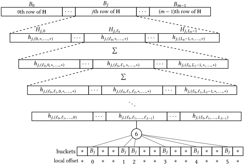
## Diagram: Hierarchical Data Decomposition and Bucket Mapping ### Overview The image is a technical diagram illustrating a multi-level hierarchical decomposition of a data structure, likely a matrix or hash table, culminating in a mapping to a bucket array with local offsets. It visually represents how a high-level row of data is progressively broken down into finer-grained components through several aggregation layers before being assigned to specific storage locations. ### Components/Axes The diagram is organized into three main spatial regions: 1. **Header (Top Region):** A horizontal array of blocks representing rows of a matrix `H`. * **Labels:** `B₀`, `Bⱼ`, `Bₘ₋₁`. * **Descriptions:** "0th row of H", "jth row of H", "(m-1)th row of H". * **Spatial Grounding:** This array spans the top of the diagram. Dashed lines emanate downward from the central block `Bⱼ`, indicating it is the subject of detailed expansion. 2. **Main Diagram (Central Region):** A vertical, multi-tiered breakdown of the `j`th row (`Bⱼ`). Each tier is a horizontal array of elements, with dashed lines connecting an element from the tier above to the entire array of the tier below, showing decomposition. * **Tier 1 (Directly below Header):** Array labeled `Hⱼ,₀` to `Hⱼ,L₀₋₁`. Elements are of the form `hⱼ,(₀,*,...,* )` to `hⱼ,(L₀₋₁,*,...,* )`. * **Tier 2:** Connected via a summation symbol (`Σ`) from Tier 1. Array of elements like `hⱼ,(ℓ₀,₀,*,...,* )` to `hⱼ,(ℓ₀,L₁₋₁,*,...,* )`. * **Tier 3:** Connected via another `Σ` from Tier 2. Array of elements like `hⱼ,(ℓ₀,ℓ₁,₀,*,...,* )` to `hⱼ,(ℓ₀,ℓ₁,L₂₋₁,*,...,* )`. * **Ellipsis (`⋮`):** Indicates continuation of this hierarchical pattern for an unspecified number of levels. * **Final Tier (Bottom of Central Region):** Array of elements `hⱼ,(ℓ₀,ℓ₁,...,0)` to `hⱼ,(ℓ₀,ℓ₁,...,Lλ₋₁)`. * **Node:** A circled number `6` is connected via a line to the central element `hⱼ,(ℓ₀,ℓ₁,...,Lλ₋₁)` of the final tier. 3. **Footer (Bottom Region):** A two-row table representing a bucket structure. | Label | Content (from left to right) | |-------|------------------------------| | buckets | `*`, `Bⱼ`, `*`, `*`, `Bⱼ`, `Bⱼ`, `*`, `*`, `Bⱼ`, `*`, `*`, `Bⱼ`, `*`, `*`, `Bⱼ`, `*` | | local offset | `*`, `0`, `*`, `*`, `1`, `2`, `*`, `*`, `3`, `*`, `*`, `4`, `*`, `*`, `5`, `*` | * **Spatial Grounding:** This table is at the very bottom. Lines from node `6` connect to multiple `Bⱼ` entries in the "buckets" row, indicating the mapping from the decomposed data element to its storage locations. ### Detailed Analysis * **Hierarchical Decomposition Flow:** The diagram shows a clear top-down flow. A single row `Bⱼ` of matrix `H` is first divided into `L₀` major segments (`Hⱼ,₀` to `Hⱼ,L₀₋₁`). Each segment `Hⱼ,ℓ₀` is then subdivided into `L₁` sub-segments, and this process repeats for `λ` levels (as indicated by the final index `ℓλ₋₁`). * **Data Element Notation:** The notation `hⱼ,(ℓ₀,ℓ₁,...,ℓₖ)` represents a specific data element at the `k`-th level of decomposition for the `j`-th row. The asterisks `*` in earlier tiers denote indices that are not yet specified at that level of the hierarchy. * **Aggregation Symbols:** The summation symbols (`Σ`) between tiers suggest that the elements in a lower tier are derived from or aggregated into the element of the tier above. * **Bucket Mapping:** The final, most granular element `hⱼ,(ℓ₀,ℓ₁,...,Lλ₋₁)` is linked to node `6`. This node then fans out to connect with specific entries labeled `Bⱼ` in the "buckets" array. The "local offset" row provides a sequential index (0, 1, 2, 3, 4, 5) for these `Bⱼ` entries, suggesting an ordered placement within the bucket structure. The asterisks (`*`) in the bucket array likely represent empty slots or slots belonging to other data rows (`Bᵢ` where `i ≠ j`). ### Key Observations 1. **Structured Hierarchy:** The diagram meticulously illustrates a recursive or multi-resolution breakdown of data, common in structures like hierarchical matrices, multi-level indexes, or certain hashing schemes. 2. **Selective Mapping:** Not all elements from the final decomposition tier are mapped to buckets. The connection is specifically from one element (via node `6`) to multiple, non-contiguous `Bⱼ` slots in the bucket array. 3. **Sparse Bucket Array:** The "buckets" row is sparse, with `Bⱼ` entries interspersed with asterisks, indicating a non-dense or hashed storage layout. 4. **Consistent Indexing:** The "local offset" provides a clean, sequential counter (0-5) for the `Bⱼ` entries, which may be used for addressing or retrieval within the bucket structure. ### Interpretation This diagram models a sophisticated data organization strategy, likely for efficient storage and retrieval in computational contexts such as numerical linear algebra (e.g., Hierarchical Matrices) or database indexing. * **What it demonstrates:** It shows how a large, monolithic data block (a row of `H`) is systematically fragmented into a hierarchy of smaller, more manageable pieces. This fragmentation allows for operations to be performed on specific sub-sections without processing the entire row. * **Relationships:** The flow from top to bottom represents increasing specificity. The `Σ` symbols imply that information is combined or summarized as one moves up the hierarchy. The final mapping via node `6` to the bucket array is the critical step that translates this logical, hierarchical decomposition into a physical or linear storage scheme. * **Notable Pattern/Anomaly:** The key pattern is the **one-to-many mapping** from a single leaf node in the hierarchy to multiple, spaced-apart locations in the bucket array. This is characteristic of a hashing or scattering operation, where a computed key (from the hierarchical indices `ℓ₀...ℓλ₋₁`) determines several storage addresses. The sparsity of the bucket array (`*` entries) further supports this, suggesting collision resolution or a design that trades space for faster access. The entire structure aims to balance the logical organization of complex data with the practical constraints of linear memory or storage.

## Diagram: Hierarchical Matrix Decomposition with Bucket Allocation ### Overview The diagram illustrates a hierarchical decomposition of matrix elements into "buckets" with local offsets. It shows a multi-level structure where rows of a matrix **H** are broken down into progressively refined sub-elements, ultimately mapped to buckets labeled **B₀** to **B₅** with associated local offsets (0–5). Dotted lines indicate relationships between matrix elements and their bucket assignments. --- ### Components/Axes 1. **Matrix Rows (Top Section)**: - **B₀** to **Bₘ₋₁**: Represent rows of matrix **H** (0th to (m−1)th row). - Each row contains elements like **Hⱼ,₀**, **Hⱼ,ℓ₀**, **Hⱼ,L₀−1**, with indices varying across dimensions (e.g., **hⱼ(0,*,...,*)**, **hⱼ(ℓ₀,*,...,*)**). 2. **Summation Layers (Middle Section)**: - **Σ Symbols**: Indicate aggregation operations across indices (e.g., **hⱼ(ℓ₀,ℓ₁,*,...,*)**). - Elements are grouped by increasing specificity in their index patterns (e.g., **hⱼ(ℓ₀,ℓ₁,...,L₁−1)**). 3. **Buckets and Local Offsets (Bottom Section)**: - **Buckets**: Labeled **B₀** to **B₅**, each marked with a star (*) symbol. - **Local Offsets**: Numerical values (0–5) positioned below buckets, suggesting positional identifiers within buckets. 4. **Dotted Lines**: - Connect matrix elements to buckets, implying a mapping or allocation logic (e.g., **hⱼ(ℓ₀,ℓ₁,...,L₁−1)** maps to **B₃** with offset 3). --- ### Detailed Analysis - **Matrix Element Indices**: - Elements are parameterized by indices like **ℓ₀, ℓ₁, ..., L₁−1**, which likely represent hierarchical or partitioned dimensions of **H**. - The use of **\*** in indices (e.g., **hⱼ(0,*,...,*)**) suggests wildcard or variable dimensions, possibly indicating sparsity or aggregation. - **Bucket Allocation**: - Buckets **B₀–B₅** are evenly spaced at the bottom, with local offsets 0–5 directly below them. - Dotted lines from elements to buckets imply a one-to-one or many-to-one mapping (e.g., **hⱼ(ℓ₀,ℓ₁,...,L₁−1)** maps to **B₃** with offset 3). - **Hierarchical Structure**: - The diagram progresses from coarse (entire rows **B₀–Bₘ₋₁**) to fine-grained (bucket-specific elements **hⱼ(ℓ₀,ℓ₁,...,L₁−1)**). - Summation symbols (**Σ**) indicate iterative refinement or aggregation across dimensions. --- ### Key Observations 1. **No Numerical Data**: The diagram lacks explicit numerical values, focusing instead on symbolic relationships and structural patterns. 2. **Consistent Labeling**: - All bucket labels (**B₀–B₅**) and offsets (0–5) are explicitly marked. - Matrix elements follow a consistent indexing convention (e.g., **Hⱼ,ℓ₀**, **Hⱼ,ℓ₁**). 3. **Spatial Grounding**: - **B₀** is top-left, **Bₘ₋₁** is top-right. - Buckets are bottom-aligned, with offsets directly beneath them. 4. **Legend Ambiguity**: - No explicit legend is present, but the star (*) symbol and offset numbering likely serve as implicit identifiers. --- ### Interpretation This diagram represents a **hierarchical data structure** for organizing matrix elements into optimized storage or computation units (buckets). Key insights: - **Efficient Access**: By decomposing **H** into buckets with local offsets, the structure may enable faster retrieval or parallel processing of sub-elements. - **Aggregation Logic**: Summation symbols (**Σ**) suggest that certain elements are precomputed or grouped for efficiency (e.g., sparse matrix operations). - **Indexing Strategy**: The use of **\*** in indices implies a flexible or adaptive partitioning scheme, possibly for handling variable-sized data or dynamic resizing. The absence of numerical values limits quantitative analysis, but the structural patterns emphasize **modularity** and **scalability** in matrix operations. This could be relevant to fields like machine learning (e.g., tensor decomposition) or distributed computing (e.g., sharding data across nodes).