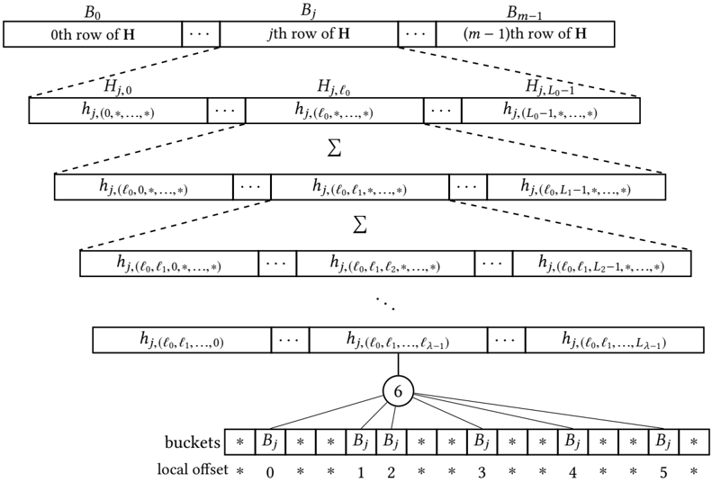
\n ## Diagram: Data Processing Flow with Bucketing ### Overview The image depicts a diagram illustrating a data processing flow, likely related to a hashing or indexing scheme. It shows a series of transformations applied to data represented as rows of 'H', culminating in a bucketing process. The diagram uses boxes to represent data structures and arrows to indicate the flow of information. ### Components/Axes The diagram consists of several key components: * **Top Row:** Represents rows of a matrix 'H', labeled as B₀, Bⱼ, ..., Bₘ₋₁. * **Intermediate Rows:** Show transformations of the data, denoted as hⱼ.(l₀,*,*), hⱼ.(l₀,l₁,*,*), etc. These rows are connected by summation symbols (Σ). * **Bottom Row:** Represents the final output, hⱼ.(l₀,l₁,..,l₂₋₁). * **Bucketing Section:** A tree-like structure at the bottom, labeled "buckets" and "local offset", with values 0 through 5. The central node is labeled "6". * **Arrows:** Indicate the flow of data and the application of summation operations. ### Detailed Analysis or Content Details The diagram shows a process that starts with rows of a matrix 'H'. Let's break down the flow: 1. **Initial Rows:** The top row represents the initial data, consisting of rows labeled B₀ through Bₘ₋₁. The subscript 'm' indicates the total number of rows. 2. **First Transformation:** The second row shows a transformation of each row of 'H', represented as hⱼ.(l₀,*,*). The 'j' likely indicates the row index, and 'l₀' represents some initial parameter. The asterisk (*) suggests that other parameters are involved but are not explicitly specified. 3. **Summation:** The summation symbol (Σ) indicates that the values in each column are summed across the rows. 4. **Iterative Transformation:** The process repeats with subsequent rows, adding more parameters (l₁, l₂, etc.) to the transformation function hⱼ.(l₀,l₁,*,*), hⱼ.(l₀,l₁,l₂,*,*), and so on. 5. **Final Output:** The bottom row represents the final transformed data, hⱼ.(l₀,l₁,..,l₂₋₁). 6. **Bucketing:** The bottom section shows a bucketing process. The "buckets" are labeled with Bⱼ, and the "local offset" ranges from 0 to 5. The central node labeled "6" suggests that the bucketing process involves a modulo operation or some other function that maps the transformed data to one of the six buckets. ### Key Observations * The diagram illustrates an iterative process of transformation and summation. * The parameters l₀, l₁, l₂... suggest a multi-dimensional indexing or hashing scheme. * The bucketing process appears to distribute the transformed data into a fixed number of buckets (6 in this case). * The asterisk (*) indicates that there are other parameters involved in the transformation function that are not explicitly shown. ### Interpretation The diagram likely represents a hashing or indexing algorithm. The initial rows of 'H' represent the input data. The iterative transformations and summations are used to generate a hash value or index. The bucketing process then distributes the data into a fixed number of buckets based on the hash value. The use of parameters l₀, l₁, l₂... suggests that the algorithm is designed to handle multi-dimensional data or to provide a more robust hashing function. The asterisk (*) indicates that the algorithm may involve additional parameters or operations that are not explicitly shown in the diagram. The central node labeled "6" in the bucketing section suggests that the hash value is modulo 6, resulting in 6 buckets. This is a common technique for distributing data evenly across a fixed number of buckets. The diagram provides a high-level overview of the algorithm and does not specify the exact details of the transformation function or the bucketing process. However, it provides a clear understanding of the overall flow of data and the key components involved. The diagram is a conceptual representation and does not contain specific numerical data. It is a visual explanation of a process.