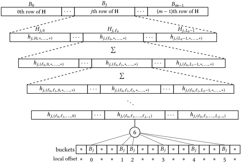
## Diagram: Hierarchical Matrix Decomposition with Bucket Allocation ### Overview The diagram illustrates a hierarchical decomposition of matrix elements into "buckets" with local offsets. It shows a multi-level structure where rows of a matrix **H** are broken down into progressively refined sub-elements, ultimately mapped to buckets labeled **B₀** to **B₅** with associated local offsets (0–5). Dotted lines indicate relationships between matrix elements and their bucket assignments. --- ### Components/Axes 1. **Matrix Rows (Top Section)**: - **B₀** to **Bₘ₋₁**: Represent rows of matrix **H** (0th to (m−1)th row). - Each row contains elements like **Hⱼ,₀**, **Hⱼ,ℓ₀**, **Hⱼ,L₀−1**, with indices varying across dimensions (e.g., **hⱼ(0,*,...,*)**, **hⱼ(ℓ₀,*,...,*)**). 2. **Summation Layers (Middle Section)**: - **Σ Symbols**: Indicate aggregation operations across indices (e.g., **hⱼ(ℓ₀,ℓ₁,*,...,*)**). - Elements are grouped by increasing specificity in their index patterns (e.g., **hⱼ(ℓ₀,ℓ₁,...,L₁−1)**). 3. **Buckets and Local Offsets (Bottom Section)**: - **Buckets**: Labeled **B₀** to **B₅**, each marked with a star (*) symbol. - **Local Offsets**: Numerical values (0–5) positioned below buckets, suggesting positional identifiers within buckets. 4. **Dotted Lines**: - Connect matrix elements to buckets, implying a mapping or allocation logic (e.g., **hⱼ(ℓ₀,ℓ₁,...,L₁−1)** maps to **B₃** with offset 3). --- ### Detailed Analysis - **Matrix Element Indices**: - Elements are parameterized by indices like **ℓ₀, ℓ₁, ..., L₁−1**, which likely represent hierarchical or partitioned dimensions of **H**. - The use of **\*** in indices (e.g., **hⱼ(0,*,...,*)**) suggests wildcard or variable dimensions, possibly indicating sparsity or aggregation. - **Bucket Allocation**: - Buckets **B₀–B₅** are evenly spaced at the bottom, with local offsets 0–5 directly below them. - Dotted lines from elements to buckets imply a one-to-one or many-to-one mapping (e.g., **hⱼ(ℓ₀,ℓ₁,...,L₁−1)** maps to **B₃** with offset 3). - **Hierarchical Structure**: - The diagram progresses from coarse (entire rows **B₀–Bₘ₋₁**) to fine-grained (bucket-specific elements **hⱼ(ℓ₀,ℓ₁,...,L₁−1)**). - Summation symbols (**Σ**) indicate iterative refinement or aggregation across dimensions. --- ### Key Observations 1. **No Numerical Data**: The diagram lacks explicit numerical values, focusing instead on symbolic relationships and structural patterns. 2. **Consistent Labeling**: - All bucket labels (**B₀–B₅**) and offsets (0–5) are explicitly marked. - Matrix elements follow a consistent indexing convention (e.g., **Hⱼ,ℓ₀**, **Hⱼ,ℓ₁**). 3. **Spatial Grounding**: - **B₀** is top-left, **Bₘ₋₁** is top-right. - Buckets are bottom-aligned, with offsets directly beneath them. 4. **Legend Ambiguity**: - No explicit legend is present, but the star (*) symbol and offset numbering likely serve as implicit identifiers. --- ### Interpretation This diagram represents a **hierarchical data structure** for organizing matrix elements into optimized storage or computation units (buckets). Key insights: - **Efficient Access**: By decomposing **H** into buckets with local offsets, the structure may enable faster retrieval or parallel processing of sub-elements. - **Aggregation Logic**: Summation symbols (**Σ**) suggest that certain elements are precomputed or grouped for efficiency (e.g., sparse matrix operations). - **Indexing Strategy**: The use of **\*** in indices implies a flexible or adaptive partitioning scheme, possibly for handling variable-sized data or dynamic resizing. The absence of numerical values limits quantitative analysis, but the structural patterns emphasize **modularity** and **scalability** in matrix operations. This could be relevant to fields like machine learning (e.g., tensor decomposition) or distributed computing (e.g., sharding data across nodes).