## Line Chart: Test-Time Compute Scaling w.r.t. Problem Difficulty ### Overview The image is a line chart that illustrates the relationship between problem difficulty and the average number of tokens, along with the standard deviation. The x-axis represents problem difficulty, measured by Pass@1, ranging from easy to difficult (1.0 to 0.0). The y-axis represents the average number of thinking tokens. The chart displays a blue line representing the average tokens and a gray area representing the standard deviation. ### Components/Axes * **Title:** Test-Time Compute Scaling w.r.t. Problem Difficulty * **X-Axis:** * **Label:** Problem Difficulty (Measured by Pass@1, Easy → Difficult) * **Scale:** 1.0, 0.8, 0.6, 0.4, 0.2, 0.0 * **Y-Axis:** * **Label:** Avg. Thinking Tokens * **Scale:** 8000, 10000, 12000, 14000, 16000, 18000 * **Legend:** Located in the top-left corner. * **Blue Line:** Avg. Tokens * **Gray Area:** Std. Deviation ### Detailed Analysis * **Avg. Tokens (Blue Line):** * The line starts at approximately 8500 tokens at a problem difficulty of 1.0. * It rises to approximately 10500 tokens around 0.9 difficulty. * It dips to approximately 8800 tokens around 0.8 difficulty. * It rises to approximately 11500 tokens around 0.7 difficulty. * It dips to approximately 10800 tokens around 0.6 difficulty. * It rises to approximately 12500 tokens around 0.5 difficulty. * It dips to approximately 10800 tokens around 0.4 difficulty. * It rises to approximately 13000 tokens around 0.3 difficulty. * It dips to approximately 9500 tokens around 0.2 difficulty. * It rises to approximately 16000 tokens around 0.1 difficulty. * It ends at approximately 15500 tokens at a problem difficulty of 0.0. * Overall trend: The average number of tokens generally increases as the problem difficulty increases (from 1.0 to 0.0). The line fluctuates significantly. * **Std. Deviation (Gray Area):** * The gray area represents the standard deviation around the average number of tokens. The width of the gray area indicates the variability in the number of tokens for a given problem difficulty. * The standard deviation appears to be relatively small at the extreme ends of the problem difficulty spectrum (1.0 and 0.0) and larger in the middle (around 0.4-0.6). ### Key Observations * The average number of tokens generally increases as the problem difficulty increases (from easy to difficult). * There are significant fluctuations in the average number of tokens across different problem difficulties. * The standard deviation varies across different problem difficulties, suggesting that the variability in the number of tokens is not constant. ### Interpretation The chart suggests that more difficult problems (lower Pass@1 values) generally require a larger number of tokens, indicating a higher computational load or more complex processing. The fluctuations in the average number of tokens may be due to variations in the types of problems or the specific algorithms used to solve them. The standard deviation provides insight into the consistency of the token count for problems of similar difficulty. A larger standard deviation suggests greater variability in the computational resources required for problems within that difficulty range.

\n ## Line Chart: Test-Time Compute Scaling w.r.t. Problem Difficulty ### Overview This line chart illustrates the relationship between problem difficulty and the average number of thinking tokens required during test-time compute. The chart also displays the standard deviation around the average. Problem difficulty is measured by Pass@1, where higher values indicate easier problems and lower values indicate more difficult problems. ### Components/Axes * **Title:** "Test-Time Compute Scaling w.r.t. Problem Difficulty" (Top-center) * **X-axis:** "Problem Difficulty (Measured by Pass@1, Easy → Difficult)" - Scale ranges from 1.0 (left) to 0.0 (right). * **Y-axis:** "Avg. Thinking Tokens" - Scale ranges from 8000 (bottom) to 18000 (top). * **Legend:** Located in the top-left corner. * "Avg. Tokens" - Represented by a solid blue line. * "Std. Deviation" - Represented by a shaded grey area. ### Detailed Analysis The chart displays two data series: the average number of tokens and the standard deviation. **Avg. Tokens (Blue Line):** The blue line exhibits a complex, oscillating pattern. * At x = 1.0, the average tokens is approximately 9,500. * The line initially increases, reaching a peak of approximately 12,500 tokens at x = 0.8. * It then decreases to around 11,000 tokens at x = 0.7. * The line fluctuates between approximately 11,000 and 16,000 tokens for x values between 0.7 and 0.3. * A peak of approximately 16,500 tokens is observed at x = 0.25. * Finally, the line decreases to approximately 15,000 tokens at x = 0.0. **Std. Deviation (Grey Shaded Area):** The standard deviation varies significantly across the range of problem difficulties. * At x = 1.0, the standard deviation is approximately 2,000 tokens. * The standard deviation generally increases as problem difficulty decreases (x values decrease). * The standard deviation reaches its maximum value (approximately 4,000 tokens) around x = 0.2. * The standard deviation decreases slightly as x approaches 0.0, settling around 3,000 tokens. ### Key Observations * The average number of tokens required appears to be higher for more difficult problems (lower Pass@1 values). * The standard deviation is larger for more difficult problems, indicating greater variability in the number of tokens needed. * The oscillating pattern of the average tokens suggests that the relationship between problem difficulty and compute is not linear. There are likely specific problem types within each difficulty level that require varying amounts of compute. * The standard deviation is consistently above zero, indicating that there is always some degree of variability in the compute required for a given problem difficulty. ### Interpretation The data suggests that as problem difficulty increases (Pass@1 decreases), the average compute required (measured in tokens) also tends to increase. However, this relationship is not straightforward; there are fluctuations indicating that other factors beyond overall difficulty influence compute requirements. The increasing standard deviation with difficulty suggests that predicting compute needs for harder problems is more challenging. This could be due to the increased complexity of these problems, leading to a wider range of solution paths and compute demands. The oscillations in the average tokens line could be indicative of different categories of problems within each difficulty level. For example, some problems might require more reasoning steps, while others might require more memory access, leading to variations in token usage. Further analysis, potentially categorizing problems by type, could reveal more nuanced insights into the relationship between problem difficulty and compute scaling. The chart highlights the importance of considering both average compute requirements and variability when designing and optimizing systems for problem-solving tasks.

\n ## Line Chart with Confidence Band: Test-Time Compute Scaling w.r.t. Problem Difficulty ### Overview The image is a line chart titled "Test-Time Compute Scaling w.r.t. Problem Difficulty." It visualizes the relationship between the average number of "thinking tokens" used by a system and the difficulty of the problem it is solving. The chart includes a central trend line and a shaded region representing variability. ### Components/Axes * **Title:** "Test-Time Compute Scaling w.r.t. Problem Difficulty" (Top center). * **X-Axis (Horizontal):** * **Label:** "Problem Difficulty (Measured by Pass@1, Easy → Difficult)" * **Scale:** Reversed linear scale, running from 1.0 on the left to 0.0 on the right. * **Major Tick Marks:** 1.0, 0.8, 0.6, 0.4, 0.2, 0.0. * **Interpretation:** A higher Pass@1 score (closer to 1.0) indicates an easier problem. The axis explicitly states that difficulty increases from left (Easy) to right (Difficult). * **Y-Axis (Vertical):** * **Label:** "Avg. Thinking Tokens" * **Scale:** Linear scale, ranging from 8000 to 18000. * **Major Tick Marks:** 8000, 10000, 12000, 14000, 16000, 18000. * **Legend:** Positioned in the top-left corner of the plot area. * **Blue Line:** Labeled "Avg. Tokens" * **Gray Shaded Area:** Labeled "Std. Deviation" ### Detailed Analysis **Data Series: "Avg. Tokens" (Blue Line)** * **Trend:** The line exhibits a clear, oscillatory upward trend as problem difficulty increases (moving from left to right on the x-axis). It is not a smooth increase but a series of peaks and valleys. * **Approximate Data Points (at major x-axis ticks):** * Difficulty 1.0 (Easiest): ~8,400 tokens. * Difficulty 0.8: ~11,500 tokens (local peak). * Difficulty 0.6: ~10,700 tokens (local valley). * Difficulty 0.5 (midpoint between 0.6 and 0.4): ~13,900 tokens (major peak). * Difficulty 0.4: ~10,500 tokens (local valley). * Difficulty 0.3: ~15,500 tokens (major peak). * Difficulty 0.2: ~11,000 tokens (local valley). * Difficulty 0.15: ~16,200 tokens (highest peak). * Difficulty 0.0 (Most Difficult): ~15,300 tokens. **Data Series: "Std. Deviation" (Gray Shaded Area)** * **Description:** This band represents the standard deviation around the average token count. Its width indicates the variability or spread of the data at each difficulty level. * **Observation:** The band is relatively narrow for easier problems (left side, difficulty ~1.0 to 0.7). It becomes dramatically wider and more irregular for harder problems (right side, difficulty < 0.5), indicating much higher variance in the number of tokens used. The widest points of the band appear to align with the peaks in the average line, particularly around difficulties 0.5, 0.3, and 0.15. ### Key Observations 1. **Oscillatory Scaling:** The average compute (tokens) does not increase monotonically with difficulty. Instead, it follows a wave-like pattern with pronounced peaks and valleys. 2. **Increasing Variance:** The standard deviation grows substantially as problems become harder. This suggests that for difficult problems, the system's token usage is highly unpredictable—sometimes using a moderate amount and sometimes a very large amount. 3. **Peak Alignment:** The highest average token usage (peaks) occurs at specific, intermediate difficulty levels (e.g., ~0.5, ~0.3, ~0.15), not necessarily at the absolute hardest difficulty (0.0). 4. **Reversed Axis:** The x-axis is intentionally reversed to map "Easy" to the left and "Difficult" to the right, which is a common but important convention to note for correct interpretation. ### Interpretation This chart demonstrates that the computational effort (measured in thinking tokens) required by the system scales in a non-linear and non-smooth fashion with problem difficulty. The oscillatory pattern suggests there may be distinct "regimes" or classes of problems where the system's reasoning process requires significantly more or less compute, even within a narrow band of measured difficulty. The most critical insight is the exploding standard deviation for hard problems. This indicates a lack of robustness or consistency. While the *average* token count increases, the *experience* for any single hard problem is highly variable. This could mean the system sometimes finds an efficient solution path and other times gets stuck in a computationally expensive loop, leading to the wide spread. The peaks in average usage might correspond to problem types that are particularly challenging for the system's architecture, forcing extensive "thinking" regardless of the precise Pass@1 score. The data implies that managing performance on the hardest problems requires addressing this high variance, not just the average case.

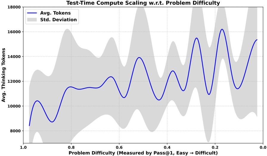
## Line Chart: Test-Time Compute Scaling w.r.t. Problem Difficulty ### Overview The chart illustrates the relationship between problem difficulty (measured by Pass@1, with 1.0 representing "Easy" and 0.0 representing "Difficult") and the average number of thinking tokens required, along with the standard deviation of token usage. The x-axis decreases from 1.0 (easy) to 0.0 (difficult), while the y-axis ranges from 8,000 to 18,000 tokens. A blue line represents the average tokens, and a gray shaded area indicates the standard deviation. ### Components/Axes - **X-Axis**: "Problem Difficulty (Measured by Pass@1, Easy → Difficult)" - Scale: 1.0 (left) to 0.0 (right), with markers at 1.0, 0.8, 0.6, 0.4, 0.2, 0.0. - **Y-Axis**: "Avg. Thinking Tokens" - Scale: 8,000 (bottom) to 18,000 (top), with markers at 8,000, 10,000, 12,000, 14,000, 16,000, 18,000. - **Legend**: - Top-left corner. - Blue line: "Avg. Tokens" - Gray shaded area: "Std. Deviation" - **Grid**: Dotted lines for alignment. ### Detailed Analysis - **Avg. Tokens (Blue Line)**: - The line starts at ~8,500 tokens at x=1.0 (easy) and increases to ~16,000 tokens at x=0.0 (difficult). - Peaks occur at x=0.6 (~12,000 tokens), x=0.4 (~13,000 tokens), x=0.2 (~15,000 tokens), and x=0.0 (~16,000 tokens). - The trend shows a general upward slope as problem difficulty decreases (x-axis moves right). - **Std. Deviation (Gray Shaded Area)**: - The shaded area is widest at x=1.0 (~2,000 tokens) and narrowest at x=0.0 (~1,000 tokens). - Variability decreases as problem difficulty increases (x-axis moves left). ### Key Observations 1. **Inverse Relationship**: As problem difficulty decreases (x-axis moves right), the average number of tokens required increases. 2. **Peaks in Token Usage**: Notable spikes in token usage occur at x=0.6, 0.4, 0.2, and 0.0, suggesting specific difficulty thresholds where compute scaling is more pronounced. 3. **Standard Deviation Trends**: The standard deviation (gray area) is largest at higher difficulty levels (x=1.0) and smallest at lower difficulty levels (x=0.0), indicating greater variability in token usage for easier problems. ### Interpretation The data suggests that **test-time compute scaling is inversely related to problem difficulty**. Easier problems (higher x-values) require fewer tokens on average but exhibit higher variability in token usage, while harder problems (lower x-values) demand more tokens with tighter variability. The peaks in token usage at specific difficulty levels (e.g., x=0.6, 0.4) may indicate critical points where the model's computational demands spike, possibly due to complex reasoning or resource-intensive operations. The narrowing standard deviation at lower difficulty levels implies that the model's performance becomes more consistent as problems become harder, potentially reflecting optimized or constrained processing strategies. **Note**: The x-axis direction (1.0 → 0.0) is unconventional, as difficulty typically increases from 0 to 1. This reversal may reflect a specific metric (e.g., Pass@1 score) where higher values correspond to easier problems.