\n
## Log-Log Plot Comparison: Energy To Solution for N=100 and N=800
### Overview
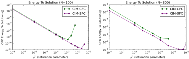
The image displays two side-by-side log-log plots comparing the "Energy To Solution" (in Joules) as a function of a "saturation parameter" (q²) for two different methods (CIM-CFC and CIM-SFC) at two different problem sizes (N=100 and N=800). The plots illustrate how the computational energy required to find a solution changes with the saturation parameter.
### Components/Axes
* **Plot Titles:**
* Left Plot: `Energy To Solution (N=100)`
* Right Plot: `Energy To Solution (N=800)`
* **X-Axis (Both Plots):**
* Label: `q² (saturation parameter)`
* Scale: Logarithmic.
* Range: Approximately `10⁻⁸` to `10⁻¹`.
* Major Ticks: `10⁻⁸`, `10⁻⁷`, `10⁻⁶`, `10⁻⁵`, `10⁻⁴`, `10⁻³`, `10⁻²`, `10⁻¹`.
* **Y-Axis (Left Plot - N=100):**
* Label: `CFO Energy To Solution (J)`
* Scale: Logarithmic.
* Range: Approximately `10⁻¹¹` to `10⁻⁴`.
* Major Ticks: `10⁻¹¹`, `10⁻¹⁰`, `10⁻⁹`, `10⁻⁸`, `10⁻⁷`, `10⁻⁶`, `10⁻⁵`, `10⁻⁴`.
* **Y-Axis (Right Plot - N=800):**
* Label: `CFO Energy To Solution (J)`
* Scale: Logarithmic.
* Range: Approximately `10⁻⁶` to `10²`.
* Major Ticks: `10⁻⁶`, `10⁻⁵`, `10⁻⁴`, `10⁻³`, `10⁻²`, `10⁻¹`, `10⁰`, `10¹`, `10²`.
* **Legend (Both Plots, Top-Right Corner):**
* `CIM-CFC`: Represented by a green line with circular markers.
* `CIM-SFC`: Represented by a purple line with circular markers.
### Detailed Analysis
**Left Plot (N=100):**
* **Trend Verification:** Both data series show a strong, nearly linear downward trend on the log-log scale for low to moderate values of q², indicating a power-law relationship where energy decreases as q² increases.
* **CIM-CFC (Green):**
* Starts at approximately `10⁻⁴ J` at `q² ≈ 10⁻⁸`.
* Decreases steadily to a minimum of approximately `10⁻¹⁰ J` at `q² ≈ 10⁻³`.
* Exhibits a sharp, significant increase (an anomaly) after `q² ≈ 10⁻³`, rising to approximately `10⁻⁷ J` at `q² ≈ 10⁻²`.
* **CIM-SFC (Purple):**
* Starts at approximately `10⁻⁴ J` at `q² ≈ 10⁻⁸`, nearly overlapping with CIM-CFC initially.
* Continues a steady, monotonic decrease across the entire range.
* Reaches its lowest point of approximately `10⁻¹¹ J` at `q² ≈ 10⁻²`.
* Shows a slight upturn at the final data point (`q² ≈ 10⁻¹`), rising to approximately `10⁻¹⁰ J`.
**Right Plot (N=800):**
* **Trend Verification:** Similar to the N=100 case, both series show a strong downward trend for low q². The overall energy scale is significantly higher (by several orders of magnitude) than for N=100.
* **CIM-CFC (Green):**
* Starts at approximately `10¹ J` at `q² ≈ 10⁻⁸`.
* Decreases to a minimum of approximately `10⁻⁴ J` at `q² ≈ 10⁻³`.
* Again shows a sharp increase after the minimum, rising to approximately `10⁻³ J` at `q² ≈ 10⁻²`.
* **CIM-SFC (Purple):**
* Starts at approximately `10¹ J` at `q² ≈ 10⁻⁸`.
* Decreases monotonically and more steeply than CIM-CFC for most of the range.
* Reaches a minimum of approximately `10⁻⁶ J` at `q² ≈ 10⁻²`.
* Exhibits a very sharp upturn at the final data point (`q² ≈ 10⁻¹`), rising to approximately `10⁻⁴ J`.
### Key Observations
1. **Scaling with N:** Increasing the problem size from N=100 to N=800 increases the required energy by approximately 5-6 orders of magnitude across the board.
2. **Method Comparison:** For both N values, the CIM-SFC method (purple) consistently achieves a lower minimum energy than the CIM-CFC method (green). The minimum for CIM-SFC occurs at a higher q² value (`~10⁻²`) compared to CIM-CFC (`~10⁻³`).
3. **Instability at High q²:** Both methods, but most dramatically CIM-CFC, show a loss of performance (increasing energy) at high saturation parameters (q² > 10⁻³). This suggests an optimal operating range for the saturation parameter.
4. **Power-Law Behavior:** The initial linear descent on the log-log plots for both methods and both N values strongly suggests a relationship of the form `Energy ∝ (q²)^k`, where `k` is a negative exponent.
### Interpretation
The data demonstrates a clear trade-off between the saturation parameter (q²) and the computational energy required to solve the problem. Initially, increasing saturation (higher q²) dramatically reduces the energy cost, following a power-law scaling. This is likely because a higher saturation parameter allows the algorithm to make more significant progress per step.
However, there is a critical point (around q² = 10⁻³ for CIM-CFC and q² = 10⁻² for CIM-SFC) beyond which further increasing saturation becomes detrimental, causing the energy cost to rise. This could indicate the onset of numerical instability, overshooting, or a breakdown in the algorithm's convergence properties when the saturation is too high.
The CIM-SFC method appears more robust and efficient than CIM-CFC for this task. It not only reaches a lower absolute energy minimum but also maintains its improving trend up to a higher saturation value before degrading. The significant increase in energy with problem size (N) highlights the computational challenge of scaling these methods. The plots serve as a guide for selecting an optimal q² to minimize energy consumption for a given problem size and method.