## Line Graph: Relationship Between C^(c)(T) and T for Varying x Values
### Overview
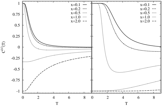
The image displays a dual-panel line graph comparing the relationship between C^(c)(T) (y-axis) and T (x-axis) for five distinct x values (0.1, 0.2, 0.5, 1.0, 2.0). The left panel shows T ≥ 0, while the right panel shows T ≤ 0. Curves are differentiated by line styles (solid, dashed, dotted, etc.) corresponding to x values in the legend.
### Components/Axes
- **Y-axis**: Labeled "C^(c)(T)" with values ranging from -1 to 1 in 0.25 increments.
- **X-axis (Left Panel)**: Labeled "T" with values from 0 to 8 in increments of 2.
- **X-axis (Right Panel)**: Labeled "T" with values from -8 to 0 in increments of 2.
- **Legend**: Located on the right side of both panels, listing x values with line styles:
- x=0.1: Solid line
- x=0.2: Dashed line
- x=0.5: Dotted line
- x=1.0: Dash-dot line
- x=2.0: Double-dash line
### Detailed Analysis
#### Left Panel (T ≥ 0)
- All curves start near C^(c)(T) = 1 at T=0 and monotonically decrease as T increases.
- **x=0.1** (solid): Highest initial value (~1) and slowest decline, ending near -0.25 at T=8.
- **x=2.0** (double-dash): Lowest initial value (~0.75) and steepest decline, ending near -0.75 at T=8.
- Intermediate x values (0.2–1.0) show intermediate slopes and terminal values.
#### Right Panel (T ≤ 0)
- All curves start near C^(c)(T) = -1 at T=-8 and monotonically increase as T approaches 0.
- **x=0.1** (solid): Lowest initial value (~-1) and slowest ascent, ending near 0.25 at T=0.
- **x=2.0** (double-dash): Highest initial value (~-0.75) and steepest ascent, ending near 0.75 at T=0.
- Intermediate x values (0.2–1.0) show intermediate slopes and terminal values.
### Key Observations
1. **Symmetry**: The left and right panels exhibit inverse behavior, with curves in the right panel mirroring the left panel's trends but inverted in sign.
2. **x Parameter Effect**: Higher x values correlate with steeper slopes and more extreme C^(c)(T) values in both panels.
3. **Asymptotic Behavior**: Curves approach horizontal asymptotes at T=±8, suggesting saturation effects.
4. **Discontinuity at T=0**: No curves connect across the two panels, indicating a potential phase transition or boundary condition.
### Interpretation
The graph demonstrates a **nonlinear, antisymmetric relationship** between C^(c)(T) and T modulated by x. The inverse trends in positive/negative T suggest a system with **direction-dependent sensitivity** to x. Higher x values amplify the magnitude of C^(c)(T) changes, implying x acts as a **coupling constant** or **control parameter**. The lack of continuity at T=0 may indicate a **phase boundary** or **singularity** in the system's behavior. This could model phenomena like **magnetic susceptibility** in alternating fields or **viscous damping** with directional dependence.