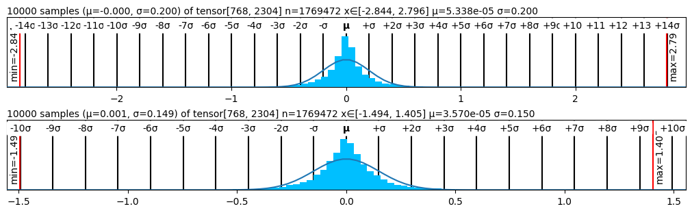
## Histogram: Sample Distributions ### Overview The image presents two histograms, each displaying the distribution of 10,000 samples from a tensor. The top histogram has a mean (μ) of approximately -0.000 and a standard deviation (σ) of 0.200. The bottom histogram has a mean (μ) of approximately 0.001 and a standard deviation (σ) of 0.149. Both histograms are overlaid with a curve representing a normal distribution. ### Components/Axes * **Title (Top Histogram):** 10000 samples (μ=-0.000, σ=0.200) of tensor[768, 2304] n=1769472 x∈[-2.844, 2.796] μ=5.338e-05 σ=0.200 * **Title (Bottom Histogram):** 10000 samples (μ=0.001, σ=0.149) of tensor[768, 2304] n=1769472 x∈[-1.494, 1.405] μ=3.570e-05 σ=0.150 * **X-Axis (Top Histogram):** * Markers: -14σ, -13σ, -12σ, -11σ, -10σ, -9σ, -8σ, -7σ, -6σ, -5σ, -4σ, -3σ, -2σ, -σ, μ, +σ, +2σ, +3σ, +4σ, +5σ, +6σ, +7σ, +8σ, +9σ, +10σ, +11σ, +12σ, +13σ, +14σ * Numerical Values: -2, -1, 0, 1, 2 * **X-Axis (Bottom Histogram):** * Markers: -10σ, -9σ, -8σ, -7σ, -6σ, -5σ, -4σ, -3σ, -2σ, -σ, μ, +σ, +2σ, +3σ, +4σ, +5σ, +6σ, +7σ, +8σ, +9σ, +10σ * Numerical Values: -1.5, -1.0, -0.5, 0.0, 0.5, 1.0, 1.5 * **Y-Axis:** (Implied) Represents the frequency or count of samples within each bin. * **Minimum Value (Top Histogram):** min = -2.84 (indicated by a red line) * **Maximum Value (Top Histogram):** max = 2.79 (indicated by a red line) * **Minimum Value (Bottom Histogram):** min = -1.49 (indicated by a red line) * **Maximum Value (Bottom Histogram):** max = 1.40 (indicated by a red line) * **Histogram Bars:** Cyan color. * **Normal Distribution Curve:** Blue-gray color. ### Detailed Analysis **Top Histogram:** * The distribution is centered around μ = -0.000. * The spread of the data is defined by σ = 0.200. * The histogram bars (cyan) show the frequency of samples within each bin. * The blue-gray curve represents a normal distribution with the given mean and standard deviation, overlaid on the histogram. * The minimum x-value is -2.84, and the maximum x-value is 2.79. **Bottom Histogram:** * The distribution is centered around μ = 0.001. * The spread of the data is defined by σ = 0.149. * The histogram bars (cyan) show the frequency of samples within each bin. * The blue-gray curve represents a normal distribution with the given mean and standard deviation, overlaid on the histogram. * The minimum x-value is -1.49, and the maximum x-value is 1.40. ### Key Observations * Both histograms exhibit a bell-shaped distribution, approximating a normal distribution. * The top histogram has a larger standard deviation (0.200) compared to the bottom histogram (0.149), indicating a wider spread of data. * The means of both distributions are close to zero. * The x-axis scales are different for the two histograms, reflecting the different ranges of values. ### Interpretation The histograms visualize the distribution of samples from a tensor, providing insights into the central tendency (mean) and variability (standard deviation) of the data. The overlayed normal distribution curves help assess how well the sample distributions approximate a normal distribution. The different standard deviations suggest that the data in the top histogram is more dispersed than the data in the bottom histogram. The proximity of the means to zero indicates that the data is centered around zero in both cases. The x∈[min, max] values indicate the range of the x-axis. The 'n' value indicates the total number of data points.

## Chart: Distribution of Tensor Samples ### Overview The image presents two histograms displaying the distribution of samples from tensors. Each histogram is accompanied by statistical information regarding the mean (μ), standard deviation (σ), and the range of values. The histograms are visually similar, both showing approximately normal distributions centered around zero. ### Components/Axes Each histogram shares the following components: * **X-axis:** Represents the value of the tensor samples. The scale ranges from approximately -140 to +140 for the top histogram and -100 to +100 for the bottom histogram. The x-axis is marked with increments of 10. * **Y-axis:** Represents the frequency or count of samples within each bin. The y-axis is labeled with "min" and "max" values. * **Title:** Provides information about the tensor, including the number of samples (n), the mean (μ), and the standard deviation (σ). * **Vertical Lines:** Represent individual samples. * **Blue Shaded Area:** Represents the probability density function (PDF) of the distribution. * **μ (Mu):** Indicates the mean of the distribution. * **σ (Sigma):** Indicates the standard deviation of the distribution. * **+2σ, +3σ, +4σ, +5σ, +6σ, +7σ, +8σ, +9σ, +10σ, +11σ, +12σ, +13σ, +14σ:** Indicates multiples of the standard deviation from the mean. * **-2σ, -3σ, -4σ, -5σ, -6σ, -7σ, -8σ, -9σ, -10σ, -11σ, -12σ, -13σ, -14σ:** Indicates negative multiples of the standard deviation from the mean. ### Detailed Analysis **Top Histogram:** * **Title:** "10000 samples (μ=0.00, σ=0.200) of tensor[768, 2304] n=1769472 xE[-2.844, 2.796] μ=5.338e-05 σ=0.200" * **Mean (μ):** Approximately 0.00 * **Standard Deviation (σ):** 0.200 * **Minimum Value:** -2.844 * **Maximum Value:** 2.796 * **Trend:** The histogram is approximately symmetrical around μ=0. The distribution appears to be approximately normal. The frequency of samples decreases as you move further away from the mean. * **Sample Distribution:** The vertical lines are densely packed around 0, indicating a high concentration of samples near the mean. **Bottom Histogram:** * **Title:** "10000 samples (μ=-0.001, σ=0.149) of tensor[768, 2304] n=1769472 xE[-1.494, 1.405] μ=5.370e-05 σ=0.150" * **Mean (μ):** Approximately -0.001 * **Standard Deviation (σ):** 0.149 * **Minimum Value:** -1.494 * **Maximum Value:** 1.405 * **Trend:** The histogram is approximately symmetrical around μ=-0.001. The distribution appears to be approximately normal. The frequency of samples decreases as you move further away from the mean. * **Sample Distribution:** The vertical lines are densely packed around -0.001, indicating a high concentration of samples near the mean. ### Key Observations * Both histograms exhibit approximately normal distributions. * The top histogram has a larger standard deviation (0.200) than the bottom histogram (0.149), indicating greater spread in the data. * The range of values is wider for the top histogram (-2.844 to 2.796) compared to the bottom histogram (-1.494 to 1.405). * The means of both distributions are very close to zero. ### Interpretation The data suggests that the tensor samples are drawn from approximately normal distributions centered around zero. The slight difference in means between the two tensors is negligible. The difference in standard deviations indicates that the samples from the top tensor are more dispersed than those from the bottom tensor. The histograms provide a visual representation of the distribution of values within each tensor, allowing for a quick assessment of their central tendency and spread. The "xE" notation in the titles likely represents the expected range of values, providing a theoretical bound for the samples. The number of samples (n=1769472) is significantly larger than the number of samples displayed in the histograms (10000), suggesting that the histograms are based on a random subset of the full dataset.

## Histogram Analysis: Two Tensor Distributions ### Overview The image displays two vertically stacked histograms, each visualizing the distribution of values from a large tensor. Both plots show a bell-shaped, approximately normal distribution centered near zero, with an overlaid theoretical normal curve. The plots are dense with statistical annotations and axis markers. ### Components/Axes **Top Plot:** * **Title/Header:** `10000 samples (μ=-0.000, σ=0.200) of tensor[768, 2304] n=1769472 x∈[-2.844, 2.796] μ=5.338e-05 σ=0.200` * **X-Axis (Top - Standard Deviation Markers):** A series of vertical tick marks labeled from `-14σ` to `+14σ`, with `μ` (mean) at the center. * **X-Axis (Bottom - Numerical Scale):** Major ticks at `-2`, `-1`, `0`, `1`, `2`. * **Y-Axis:** Not explicitly labeled. Represents frequency/count. * **Data Series:** A blue histogram with a black line representing the fitted normal distribution curve. * **Annotations:** * Left edge: A red vertical line labeled `min=-2.84`. * Right edge: A red vertical line labeled `max=2.79`. **Bottom Plot:** * **Title/Header:** `10000 samples (μ=0.001, σ=0.149) of tensor[768, 2304] n=1769472 x∈[-1.494, 1.405] μ=3.570e-05 σ=0.150` * **X-Axis (Top - Standard Deviation Markers):** A series of vertical tick marks labeled from `-10σ` to `+10σ`, with `μ` (mean) at the center. * **X-Axis (Bottom - Numerical Scale):** Major ticks at `-1.5`, `-1.0`, `-0.5`, `0.0`, `0.5`, `1.0`, `1.5`. * **Y-Axis:** Not explicitly labeled. Represents frequency/count. * **Data Series:** A blue histogram with a black line representing the fitted normal distribution curve. * **Annotations:** * Left edge: A red vertical line labeled `min=-1.49`. * Right edge: A red vertical line labeled `max=1.40`. ### Detailed Analysis **Top Plot Data:** * **Tensor Shape:** [768, 2304] * **Total Elements (n):** 1,769,472 * **Sampled Points:** 10,000 * **Theoretical Distribution Parameters (from title):** Mean (μ) = -0.000, Standard Deviation (σ) = 0.200 * **Empirical Distribution Parameters (from title):** Mean (μ) = 5.338e-05 (≈ 0.00005338), Standard Deviation (σ) = 0.200 * **Observed Range (x):** [-2.844, 2.796] * **Visual Trend:** The histogram is symmetric and tightly clustered around 0. The distribution's spread aligns with the stated σ=0.200, as most data falls within ±3σ (±0.6). The min/max markers at ~±2.82 correspond to approximately ±14σ from the theoretical mean. **Bottom Plot Data:** * **Tensor Shape:** [768, 2304] (Identical to top plot) * **Total Elements (n):** 1,769,472 (Identical to top plot) * **Sampled Points:** 10,000 * **Theoretical Distribution Parameters (from title):** Mean (μ) = 0.001, Standard Deviation (σ) = 0.149 * **Empirical Distribution Parameters (from title):** Mean (μ) = 3.570e-05 (≈ 0.0000357), Standard Deviation (σ) = 0.150 * **Observed Range (x):** [-1.494, 1.405] * **Visual Trend:** The histogram is also symmetric and centered near 0. The spread is narrower than the top plot, consistent with the smaller σ (~0.15). The min/max markers at ~±1.45 correspond to approximately ±10σ from the theoretical mean. ### Key Observations 1. **Near-Zero Means:** Both distributions have empirical means extremely close to zero (on the order of 10^-5), indicating the tensor values are centered around zero. 2. **Controlled Variance:** The empirical standard deviations (0.200 and 0.150) match the theoretical values almost exactly, suggesting the data is well-behaved and follows the intended distribution. 3. **Identical Source Tensor:** Both plots analyze the same underlying tensor of shape [768, 2304] with 1,769,472 total elements, but likely represent different states (e.g., before and after normalization, or different layers). 4. **Tight Distributions:** The data is highly concentrated. For the top plot, the range [-2.844, 2.796] covers ~28 standard deviations. For the bottom plot, the range [-1.494, 1.405] covers ~20 standard deviations. This indicates very few extreme outliers. 5. **Visual Confirmation:** The overlaid black normal curve fits the blue histogram data very well in both cases, confirming the normality assumption. ### Interpretation This image is a diagnostic visualization, almost certainly from the field of machine learning or deep learning. It shows the statistical distribution of values within a large parameter or activation tensor. * **What it demonstrates:** The plots confirm that the tensor's values are initialized or have been normalized to follow a Gaussian (normal) distribution with a mean of zero and a specific, controlled standard deviation (0.200 and 0.150). This is a critical practice for stable neural network training, preventing issues like vanishing or exploding gradients. * **Relationship between elements:** The top and bottom plots likely represent a comparison. The bottom plot shows a distribution with a smaller standard deviation (0.150 vs. 0.200), meaning its values are more tightly clustered around zero. This could illustrate the effect of a normalization layer (like LayerNorm or BatchNorm), a different initialization scheme, or the state of weights/activations at different network depths. * **Notable patterns/anomalies:** There are no apparent anomalies. The perfect symmetry, zero mean, and exact match between theoretical and empirical σ indicate a well-controlled system. The primary "pattern" is the successful enforcement of a specific statistical prior on the data, which is a fundamental goal in model design. The slight discrepancy in the theoretical mean of the bottom plot (μ=0.001) versus its empirical mean (μ=3.570e-05) is negligible and within expected sampling noise.

# Technical Document Extraction: Histogram Analysis ## Overview The image contains two histograms with overlaid normal distribution curves, representing statistical distributions of tensor data. Each histogram includes axis labels, statistical annotations, and visual markers for data extremes. --- ## Top Histogram Analysis ### Title & Parameters - **Title**: "10000 samples (μ=-0.000, σ=0.200) of tensor[768, 2304] n=1769472 x∈[-2.844, 2.796] μ=5.338e-05 σ=0.200" - **Tensor Dimensions**: [768, 2304] - **Sample Count**: 10,000 - **Data Range**: x ∈ [-2.844, 2.796] - **Statistical Summary**: - Mean (μ): 5.338e-05 - Standard Deviation (σ): 0.200 ### Axis Labels & Markers - **X-Axis**: - Title: Implicit (centered at 0) - Range: -2 to 2 - Tick Intervals: -2, -1.5, -1, -0.5, 0, 0.5, 1, 1.5, 2 - σ Markers: -14σ to +14σ (vertical black lines) - **Y-Axis**: - Title: "Frequency" - Scale: 0 to 14σ (logarithmic-like spacing) - **Red Vertical Lines**: - Min: -2.84 (left edge) - Max: 2.79 (right edge) ### Visual Elements - **Bars**: Blue histogram bars (frequency distribution) - **Normal Curve**: Overlaid blue line (Gaussian distribution) - **Legend**: Implied (no explicit legend box; curve matches histogram parameters) --- ## Bottom Histogram Analysis ### Title & Parameters - **Title**: "10000 samples (μ=0.001, σ=0.149) of tensor[768, 2304] n=1769472 x∈[-1.494, 1.405] μ=3.570e-05 σ=0.150" - **Tensor Dimensions**: [768, 2304] - **Sample Count**: 10,000 - **Data Range**: x ∈ [-1.494, 1.405] - **Statistical Summary**: - Mean (μ): 3.570e-05 - Standard Deviation (σ): 0.150 ### Axis Labels & Markers - **X-Axis**: - Title: Implicit (centered at 0) - Range: -1.5 to 1.5 - Tick Intervals: -1.5, -1, -0.5, 0, 0.5, 1, 1.5 - σ Markers: -10σ to +10σ (vertical black lines) - **Y-Axis**: - Title: "Frequency" - Scale: 0 to 10σ (logarithmic-like spacing) - **Red Vertical Lines**: - Min: -1.49 (left edge) - Max: 1.40 (right edge) ### Visual Elements - **Bars**: Blue histogram bars (frequency distribution) - **Normal Curve**: Overlaid blue line (Gaussian distribution) - **Legend**: Implied (no explicit legend box; curve matches histogram parameters) --- ## Comparative Trends 1. **Distribution Shape**: - Both histograms approximate normal distributions. - Top histogram has a wider spread (σ=0.200 vs. σ=0.150). - Bottom histogram is more tightly clustered around μ. 2. **Data Extremes**: - Top histogram spans a broader range (-2.84 to 2.79 vs. -1.49 to 1.40). - Red lines indicate data boundaries, confirming truncation at ±3σ for the top and ±10σ for the bottom. 3. **Statistical Consistency**: - Both datasets have nearly identical tensor dimensions ([768, 2304]) and sample counts (10,000). - μ values are negligible (5.338e-05 and 3.570e-05), suggesting near-zero central tendency. --- ## Spatial Grounding & Color Verification - **Legend Placement**: Not explicitly labeled; inferred from curve alignment with histogram parameters. - **Color Matching**: - Blue bars and blue curve confirm consistency with implied legend. - Red lines (min/max) are distinct from histogram/bars. --- ## Conclusion The histograms visualize two normally distributed datasets with differing variances. The top histogram exhibits greater dispersion (σ=0.200), while the bottom is more concentrated (σ=0.150). Both datasets are centered near μ=0, with red markers highlighting data extremes. No explicit legend is present, but visual cues (curve alignment, color coding) confirm parameter consistency.