## Chart: Distribution of Tensor Samples
### Overview
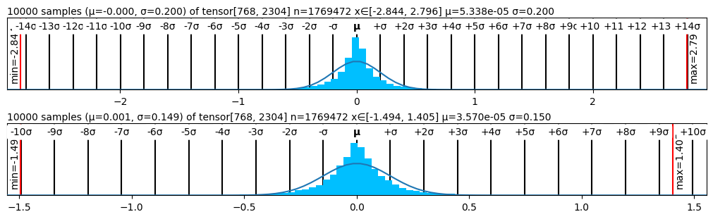
The image presents two histograms displaying the distribution of samples from tensors. Each histogram is accompanied by statistical information regarding the mean (μ), standard deviation (σ), and the range of values. The histograms are visually similar, both showing approximately normal distributions centered around zero.
### Components/Axes
Each histogram shares the following components:
* **X-axis:** Represents the value of the tensor samples. The scale ranges from approximately -140 to +140 for the top histogram and -100 to +100 for the bottom histogram. The x-axis is marked with increments of 10.
* **Y-axis:** Represents the frequency or count of samples within each bin. The y-axis is labeled with "min" and "max" values.
* **Title:** Provides information about the tensor, including the number of samples (n), the mean (μ), and the standard deviation (σ).
* **Vertical Lines:** Represent individual samples.
* **Blue Shaded Area:** Represents the probability density function (PDF) of the distribution.
* **μ (Mu):** Indicates the mean of the distribution.
* **σ (Sigma):** Indicates the standard deviation of the distribution.
* **+2σ, +3σ, +4σ, +5σ, +6σ, +7σ, +8σ, +9σ, +10σ, +11σ, +12σ, +13σ, +14σ:** Indicates multiples of the standard deviation from the mean.
* **-2σ, -3σ, -4σ, -5σ, -6σ, -7σ, -8σ, -9σ, -10σ, -11σ, -12σ, -13σ, -14σ:** Indicates negative multiples of the standard deviation from the mean.
### Detailed Analysis
**Top Histogram:**
* **Title:** "10000 samples (μ=0.00, σ=0.200) of tensor[768, 2304] n=1769472 xE[-2.844, 2.796] μ=5.338e-05 σ=0.200"
* **Mean (μ):** Approximately 0.00
* **Standard Deviation (σ):** 0.200
* **Minimum Value:** -2.844
* **Maximum Value:** 2.796
* **Trend:** The histogram is approximately symmetrical around μ=0. The distribution appears to be approximately normal. The frequency of samples decreases as you move further away from the mean.
* **Sample Distribution:** The vertical lines are densely packed around 0, indicating a high concentration of samples near the mean.
**Bottom Histogram:**
* **Title:** "10000 samples (μ=-0.001, σ=0.149) of tensor[768, 2304] n=1769472 xE[-1.494, 1.405] μ=5.370e-05 σ=0.150"
* **Mean (μ):** Approximately -0.001
* **Standard Deviation (σ):** 0.149
* **Minimum Value:** -1.494
* **Maximum Value:** 1.405
* **Trend:** The histogram is approximately symmetrical around μ=-0.001. The distribution appears to be approximately normal. The frequency of samples decreases as you move further away from the mean.
* **Sample Distribution:** The vertical lines are densely packed around -0.001, indicating a high concentration of samples near the mean.
### Key Observations
* Both histograms exhibit approximately normal distributions.
* The top histogram has a larger standard deviation (0.200) than the bottom histogram (0.149), indicating greater spread in the data.
* The range of values is wider for the top histogram (-2.844 to 2.796) compared to the bottom histogram (-1.494 to 1.405).
* The means of both distributions are very close to zero.
### Interpretation
The data suggests that the tensor samples are drawn from approximately normal distributions centered around zero. The slight difference in means between the two tensors is negligible. The difference in standard deviations indicates that the samples from the top tensor are more dispersed than those from the bottom tensor. The histograms provide a visual representation of the distribution of values within each tensor, allowing for a quick assessment of their central tendency and spread. The "xE" notation in the titles likely represents the expected range of values, providing a theoretical bound for the samples. The number of samples (n=1769472) is significantly larger than the number of samples displayed in the histograms (10000), suggesting that the histograms are based on a random subset of the full dataset.