## Diagram: Neural Network Architecture with Weights and Biases
### Overview
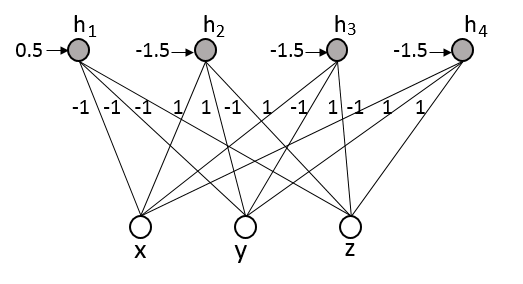
The image displays a schematic diagram of a simple feedforward neural network (or a single layer of one). It consists of two layers of nodes (neurons) connected by weighted edges. The bottom layer is the input layer, and the top layer is a hidden or output layer. Each node in the top layer receives a bias input. All text and numerical values are in English.
### Components/Axes
* **Layers:**
* **Input Layer (Bottom):** Three nodes, represented as white circles. They are labeled from left to right: **x**, **y**, **z**.
* **Hidden/Output Layer (Top):** Four nodes, represented as gray circles. They are labeled from left to right: **h₁**, **h₂**, **h₃**, **h₄**.
* **Connections (Edges):** Directed lines (arrows) connect every node in the input layer to every node in the top layer, forming a fully connected bipartite graph. Each connection has an associated numerical weight.
* **Biases:** Each node in the top layer (**h₁** to **h₄**) has an incoming arrow from the left, representing a bias input. Each bias has an associated numerical value.
### Detailed Analysis
**1. Bias Values (Applied to Top Layer Nodes):**
* Node **h₁**: Bias = **0.5**
* Node **h₂**: Bias = **-1.5**
* Node **h₃**: Bias = **-1.5**
* Node **h₄**: Bias = **-1.5**
**2. Connection Weights (From Input Layer to Top Layer):**
The weights are labeled on the lines. The pattern is consistent: all connections from a given input node to the top layer nodes share the same weight value.
* **From Input Node x:**
* To **h₁**: Weight = **-1**
* To **h₂**: Weight = **-1**
* To **h₃**: Weight = **-1**
* To **h₄**: Weight = **-1**
* **From Input Node y:**
* To **h₁**: Weight = **1**
* To **h₂**: Weight = **1**
* To **h₃**: Weight = **1**
* To **h₄**: Weight = **1**
* **From Input Node z:**
* To **h₁**: Weight = **-1**
* To **h₂**: Weight = **-1**
* To **h₃**: Weight = **-1**
* To **h₄**: Weight = **-1**
**3. Spatial Layout:**
* The four top-layer nodes (**h₁**-**h₄**) are arranged horizontally across the top of the diagram.
* The three input nodes (**x**, **y**, **z**) are arranged horizontally across the bottom.
* Bias arrows enter each **h** node from the immediate left.
* Connection lines cross the central space, creating a dense web. Lines from **x** and **z** slope upward inward, while lines from **y** go straight up.
### Key Observations
1. **Symmetry and Pattern:** The network exhibits a strong, deliberate pattern. The input node **y** has a positive weight (+1) to all top nodes, while input nodes **x** and **z** have a negative weight (-1) to all top nodes.
2. **Bias Uniformity:** Three of the four top nodes (**h₂**, **h₃**, **h₄**) share an identical bias of **-1.5**. Only **h₁** has a different bias (**0.5**).
3. **Fully Connected:** Every input is connected to every output neuron, which is standard for a dense layer.
4. **No Activation Function Shown:** The diagram depicts the linear transformation (weights and biases) but does not specify an activation function (e.g., sigmoid, ReLU) that would typically follow.
### Interpretation
This diagram represents the **linear transformation stage** of a neural network layer. The computation for each output neuron **hᵢ** is a weighted sum of the inputs plus a bias:
`hᵢ = (w_ix * x) + (w_iy * y) + (w_iz * z) + bᵢ`
Given the specific weights and biases:
* The network is configured to respond strongly to the input **y** (positive weight) and be suppressed by inputs **x** and **z** (negative weights).
* The identical parameters for **h₂**, **h₃**, and **h₄** suggest they might be redundant or part of a mechanism where multiple neurons compute the same function, possibly for increased capacity or as part of a specific architectural pattern (like an ensemble within a layer).
* The distinct bias for **h₁** makes it functionally different from the other three neurons, potentially allowing it to detect a different feature or threshold.
* This could be a simplified illustration for educational purposes, a snapshot of a network's weights after training for a specific task (e.g., a classifier where **y** is a key positive feature), or a component of a larger, more complex model. The symmetry suggests it might be a constructed example to demonstrate how weights and biases combine.