\n
## Diagram: Hidden Markov Model (HMM) / State-Space Model
### Overview
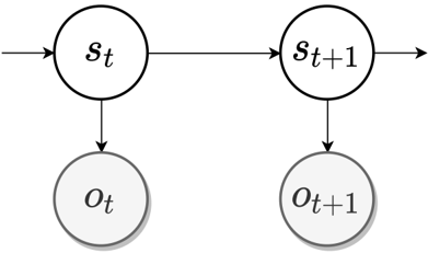
The image displays a directed graphical model, specifically a two-time-slice Bayesian network representing a Hidden Markov Model (HMM) or a general state-space model. It illustrates the probabilistic dependencies between latent state variables and observed variables across two consecutive time steps, `t` and `t+1`.
### Components/Axes
The diagram consists of four nodes (circles) and four directed edges (arrows).
**Nodes:**
1. **Top Row (Latent States):**
* **Node `s_t`**: A circle located in the upper-left quadrant. It contains the mathematical symbol `s` with a subscript `t`.
* **Node `s_{t+1}`**: A circle located in the upper-right quadrant. It contains the mathematical symbol `s` with a subscript `t+1`.
2. **Bottom Row (Observations):**
* **Node `o_t`**: A circle located directly below `s_t` in the lower-left quadrant. It contains the mathematical symbol `o` with a subscript `t`.
* **Node `o_{t+1}`**: A circle located directly below `s_{t+1}` in the lower-right quadrant. It contains the mathematical symbol `o` with a subscript `t+1`.
**Edges (Arrows):**
1. An arrow originates from the left edge of the frame and points to the left side of node `s_t`. This represents the influence from a prior state (e.g., `s_{t-1}`) or an initial state distribution.
2. A horizontal arrow points from the right side of node `s_t` to the left side of node `s_{t+1}`. This represents the state transition probability, `P(s_{t+1} | s_t)`.
3. A vertical arrow points downward from the bottom of node `s_t` to the top of node `o_t`. This represents the observation/emission probability, `P(o_t | s_t)`.
4. A vertical arrow points downward from the bottom of node `s_{t+1}` to the top of node `o_{t+1}`. This represents the observation/emission probability, `P(o_{t+1} | s_{t+1})`.
### Detailed Analysis
The diagram is a canonical representation of a first-order Markov process with hidden states.
* **Temporal Flow:** The model progresses from left to right, representing the flow of time from step `t` to `t+1`.
* **Causal Structure:**
* The state at time `t+1` (`s_{t+1}`) is conditionally dependent only on the state at the previous time `t` (`s_t`). This is the Markov property.
* The observation at any time `t` (`o_t`) is conditionally dependent only on the state at that same time (`s_t`). Observations are independent given the state sequence.
* **Visual Styling:** All nodes are simple black-outlined circles with white fill. The observation nodes (`o_t`, `o_{t+1}`) have a subtle gray drop shadow, visually distinguishing them from the state nodes. The arrows are solid black lines with arrowheads.
### Key Observations
1. **Model Type:** This is a classic Hidden Markov Model (HMM) structure. The states `s` are "hidden" or latent, while the `o` variables are the directly "observed" emissions.
2. **Time Slices:** The diagram explicitly shows two time slices, which is the minimal unit needed to illustrate the Markov property and the connection between states and observations.
3. **Missing Elements:** The diagram is abstract and does not specify:
* The dimensionality of the state or observation spaces.
* The specific probability distributions (e.g., Gaussian for continuous observations, Categorical for discrete).
* The initial state distribution (represented by the incoming arrow to `s_t`).
* Any parameters of the model.
### Interpretation
This diagram is a foundational schematic in fields like machine learning, signal processing, and computational neuroscience. It visually encodes the core assumptions of an HMM:
1. **Latent Dynamics:** The system's true condition evolves over time according to a Markov process (`s_t -> s_{t+1}`). The state `s_t` encapsulates all necessary information from the past to predict the future state.
2. **Noisy Observations:** At each time step, we do not see the true state `s_t` directly. Instead, we receive a noisy or transformed measurement `o_t` that depends probabilistically on `s_t`.
3. **Investigative Reading (Peircean):** The diagram is an *icon* of the model's conditional independence structure. It allows an expert to immediately infer the joint probability distribution factorization: `P(s_t, o_t, s_{t+1}, o_{t+1}) = P(s_t) * P(o_t | s_t) * P(s_{t+1} | s_t) * P(o_{t+1} | s_{t+1})` (with the first term implied by the incoming arrow). This structure is the basis for inference algorithms like the Forward-Backward algorithm or the Viterbi algorithm, which are used to decode the most likely hidden state sequence given a sequence of observations. The simplicity of the diagram belies the complexity of the problems it models, such as speech recognition, part-of-speech tagging, or tracking objects with noisy sensors.