## Surface Plots: Hessian vs. Random Directions ### Overview The image presents four 3D surface plots, arranged in a 2x2 grid. Each plot visualizes a function's behavior with respect to two variables, alpha (α) and beta (β). The plots are distinguished by the method used to determine the directions (Hessian vs. Random) and the range of alpha and beta values. The surface color represents the function's output, transitioning from blue (low values) to red (high values). ### Components/Axes Each plot has the following components: * **Axes:** Two axes labeled α (alpha) and β (beta) form the base of each plot. * **Surface:** A colored surface represents the function's output for different combinations of α and β. The color gradient ranges from blue to red. * **Titles:** Each plot has a title indicating the direction type (Hessian or Random) and a range for α and β. Specific labels and ranges: * **(a) Hessian directions:** α, β ∈ [-1, 1] * **(b) Random directions:** α, β ∈ [-1, 1] * **(c) Hessian directions:** α, β ∈ [-0.05, 0.05] * **(d) Random directions:** α, β ∈ [-0.05, 0.05] ### Detailed Analysis **Plot (a): Hessian directions, α, β ∈ [-1, 1]** * The surface exhibits significant undulations and variations. * There's a distinct "valley" or trough running across the surface. * The color varies considerably, indicating a wide range of function values. * The surface reaches higher values (red) at the edges, particularly along the β axis. **Plot (b): Random directions, α, β ∈ [-1, 1]** * The surface is smoother compared to plot (a). * It has a bowl-like shape, with the lowest point in the center. * The color gradient is more gradual, suggesting a smaller range of function values. * The surface also reaches higher values (red) at the edges, particularly along the β axis. **Plot (c): Hessian directions, α, β ∈ [-0.05, 0.05]** * This plot shows a zoomed-in view of the Hessian directions around the origin. * The surface is relatively smooth and bowl-shaped. * The color is predominantly blue, indicating low function values in this region. * A small inset diagram shows a further zoomed-in view of a region on the surface. The inset is connected to the main plot by several lines. **Plot (d): Random directions, α, β ∈ [-0.05, 0.05]** * This plot shows a zoomed-in view of the Random directions around the origin. * The surface is smooth and bowl-shaped, similar to plot (c). * The color is predominantly blue, indicating low function values in this region. ### Key Observations * **Direction Type:** Hessian directions (a, c) result in more complex and variable surfaces compared to Random directions (b, d). * **Range of α and β:** Reducing the range of α and β to [-0.05, 0.05] (c, d) reveals a smoother, bowl-shaped behavior near the origin for both Hessian and Random directions. * **Surface Color:** The color gradient indicates the function's output value, with blue representing lower values and red representing higher values. ### Interpretation The plots illustrate how different methods for choosing directions (Hessian vs. Random) affect the shape of the function's surface. Hessian directions, which are based on the function's curvature, lead to more complex and potentially unstable behavior, especially when considering a wider range of α and β values. Random directions, on the other hand, result in a smoother and more predictable surface. The zoomed-in views (c, d) suggest that near the origin, both methods exhibit a similar bowl-shaped behavior, indicating a local minimum. However, the behavior diverges significantly as α and β move away from the origin, as seen in plots (a) and (b). This suggests that the choice of direction method can have a significant impact on the optimization process, particularly when dealing with non-convex functions.

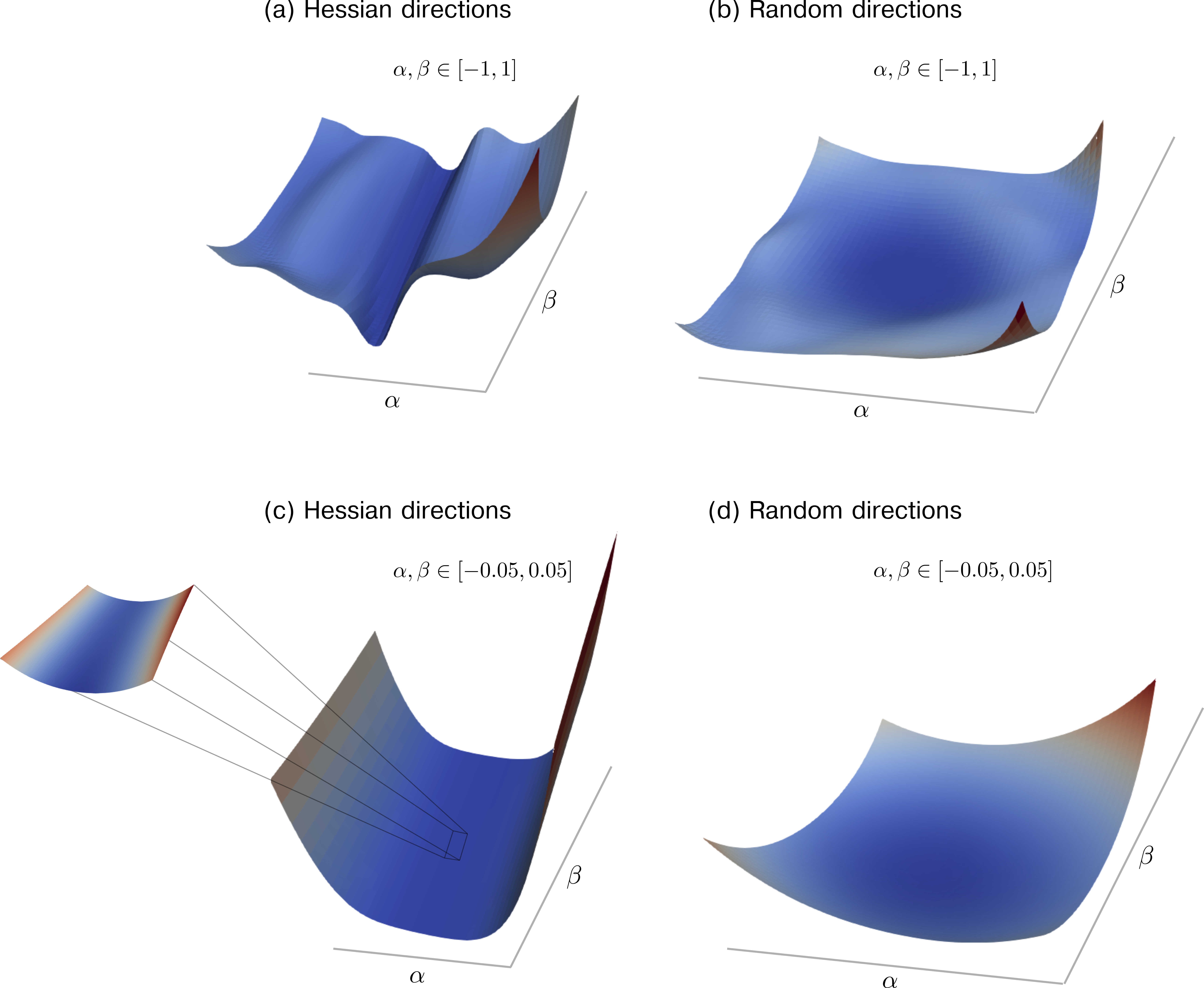
## 3D Surface Plots: Hessian and Random Directions ### Overview The image presents four 3D surface plots, arranged in a 2x2 grid. Each plot visualizes a function of two variables, α and β, with the function's value represented by the height of the surface. Two plots (a and c) use "Hessian directions" for the underlying function, while the other two (b and d) use "Random directions". Plots (a) and (b) have α, β ∈ [-1, 1], while plots (c) and (d) have α, β ∈ [-0.05, 0.05]. The color gradient on the surfaces indicates the function's value, ranging from darker blues (lower values) to lighter blues/whites (higher values). ### Components/Axes Each plot shares the following components: * **Axes:** Three orthogonal axes labeled α, β, and implicitly the function value (z-axis, height). * **Axis Ranges:** * Plots (a) and (b): α ranges from -1 to 1, β ranges from -1 to 1. * Plots (c) and (d): α ranges from -0.05 to 0.05, β ranges from -0.05 to 0.05. * **Color Scale:** A gradient from dark blue to light blue/white, representing the function's value. The exact mapping is not provided. * **Titles:** Each plot has a title indicating the direction used ("Hessian directions" or "Random directions") and a letter identifier (a, b, c, d). ### Detailed Analysis or Content Details **Plot (a): Hessian directions, α, β ∈ [-1, 1]** The surface exhibits a curved shape, rising from the bottom-left towards the top-right. The highest point appears to be near β = 1 and α = 1. The surface is relatively smooth. **Plot (b): Random directions, α, β ∈ [-1, 1]** This surface is significantly more irregular and undulating than plot (a). It has several peaks and valleys, and the overall shape is less predictable. The highest point appears to be near β = 1 and α = 0.5. **Plot (c): Hessian directions, α, β ∈ [-0.05, 0.05]** This plot shows a zoomed-in view of the Hessian direction surface. The surface is nearly flat, with a slight curvature. The highest point is near α = 0.05 and β = 0.05. **Plot (d): Random directions, α, β ∈ [-0.05, 0.05]** Similar to plot (b), this surface is irregular, but the smaller range of α and β results in a more localized and less extreme variation. The highest point appears to be near α = 0 and β = 0.05. ### Key Observations * **Directional Impact:** The "Hessian directions" (plots a and c) result in smoother, more predictable surfaces compared to the "Random directions" (plots b and d). * **Scale Effect:** Reducing the range of α and β (from [-1, 1] to [-0.05, 0.05]) significantly alters the appearance of the surfaces, making the variations less pronounced. * **Irregularity:** The "Random directions" plots consistently exhibit more irregularity and local extrema than the "Hessian directions" plots. ### Interpretation These plots likely illustrate the behavior of a function under different sampling or optimization strategies. The "Hessian directions" represent a more informed approach, leveraging second-order derivative information (the Hessian matrix) to guide the exploration of the function's landscape. This results in a smoother, more predictable path towards a potential optimum. The "Random directions," on the other hand, represent a less informed, more stochastic approach. This can lead to more erratic behavior, with the function potentially getting stuck in local optima or requiring more iterations to converge. The change in scale (from [-1, 1] to [-0.05, 0.05]) demonstrates the importance of the search space. Zooming in on a smaller region can reveal finer details and potentially uncover local optima that were not visible at a larger scale. The color gradients provide a visual representation of the function's value, allowing for a quick assessment of the function's behavior in different regions of the α-β plane. The darker blues indicate regions of lower function value, while the lighter blues/whites indicate regions of higher function value.

\n ## 3D Surface Plots: Comparison of Hessian vs. Random Direction Landscapes ### Overview The image displays four 3D surface plots arranged in a 2x2 grid. Each plot visualizes a mathematical function's surface over a two-dimensional parameter space defined by variables α (alpha) and β (beta). The plots are grouped into two categories: "Hessian directions" (left column) and "Random directions" (right column). The top row shows the landscape over a broad range, while the bottom row shows a zoomed-in view near the origin. The surfaces are colored with a gradient, where blue represents lower function values and red/brown represents higher values. ### Components/Axes * **Titles:** * Top-left (a): "Hessian directions" * Top-right (b): "Random directions" * Bottom-left (c): "Hessian directions" * Bottom-right (d): "Random directions" * **Axis Labels:** All four plots have identical axis labels. * Horizontal axis (front): α (alpha) * Horizontal axis (side): β (beta) * Vertical axis: Implied to be a function value, f(α, β), but not explicitly labeled. * **Range Annotations:** * Top Row (a & b): `α, β ∈ [-1, 1]` (indicating the parameters range from -1 to 1). * Bottom Row (c & d): `α, β ∈ [-0.05, 0.05]` (indicating a zoomed-in view near zero). * **Color Mapping (Implicit Legend):** The surface color corresponds to the vertical (function) value. The gradient transitions from deep blue (lowest points) through light blue/white to red/brown (highest points). ### Detailed Analysis **Plot (a) - Hessian directions, Range [-1, 1]:** * **Trend:** The surface is highly non-convex and complex. It features multiple local minima (deep blue valleys) and maxima (red/brown peaks). The landscape is "wrinkled" with significant curvature changes. * **Spatial Details:** A prominent deep blue valley runs diagonally from the front-left towards the center. Several sharp red peaks are visible, particularly one on the right side and another towards the back. The surface exhibits saddle points and ridges. **Plot (b) - Random directions, Range [-1, 1]:** * **Trend:** The surface is much smoother and simpler compared to (a). It resembles a broad, shallow basin or a slightly distorted paraboloid. * **Spatial Details:** The lowest point (deepest blue) is near the center of the α-β plane. The function value increases smoothly and monotonically as one moves away from the center towards the edges of the [-1, 1] domain, transitioning to red/brown at the corners. There are no visible local minima or complex features. **Plot (c) - Hessian directions, Range [-0.05, 0.05]:** * **Trend:** This is a zoomed-in view of the landscape near the origin (α=0, β=0) for the Hessian case. The surface shows a distinct saddle shape or a sharp valley. * **Spatial Details:** A deep blue valley runs through the center. The function increases sharply (to red) along one diagonal direction and more gradually along the orthogonal diagonal. An inset box with connecting lines highlights a specific rectangular region on the surface, likely to emphasize local curvature or a region of interest for further analysis. The inset is positioned in the lower-left quadrant of the plot. **Plot (d) - Random directions, Range [-0.05, 0.05]:** * **Trend:** This zoomed-in view confirms the smooth, convex nature of the random direction landscape near the origin. * **Spatial Details:** The surface is a simple, upward-opening parabolic bowl. The minimum is at the center (α=0, β=0), and the value increases uniformly in all directions, creating a smooth gradient from blue at the center to red at the edges of the small domain. ### Key Observations 1. **Complexity Dichotomy:** The most striking observation is the drastic difference in complexity between the "Hessian directions" and "Random directions" landscapes. The Hessian-based surface (a, c) is rugged with multiple optima, while the random-direction surface (b, d) is smooth and convex. 2. **Scale Invariance of Smoothness:** The smooth, convex property of the random direction landscape holds at both the large scale (b) and the very small, local scale (d). 3. **Local vs. Global Structure:** Plot (c) reveals that even in a very small neighborhood around a point, the Hessian-informed landscape can have complex, non-quadratic structure (the saddle/valley), whereas the random direction landscape (d) is purely quadratic (parabolic) locally. 4. **Color as Value Indicator:** The consistent color mapping allows for direct visual comparison of function value ranges and gradients across all four plots. ### Interpretation This figure is likely from a technical paper on optimization, machine learning, or numerical analysis, specifically discussing loss landscapes or the geometry of objective functions. * **What it Demonstrates:** The plots visually argue that exploring a function's landscape along directions informed by its Hessian matrix (which captures second-order curvature information) reveals a much more complex and challenging optimization terrain than exploring along random directions. The random directions provide a smoothed, averaged view of the landscape that hides the intricate, potentially problematic structure (like sharp valleys and multiple minima) that Hessian-based methods must navigate. * **Relationship Between Elements:** The top row provides the global context, showing the overall shape of the landscapes. The bottom row provides a local, magnified view, proving that the complexity difference persists even at microscopic scales. The inset in (c) further emphasizes the need to examine specific local features. * **Implications:** This has significant implications for optimization algorithms. It suggests that: 1. Second-order methods (using Hessian information) operate in a more complex geometric space than first-order or random search methods. 2. The apparent smoothness observed when moving in random directions might be misleading, hiding difficult curvature that can trap or slow down sophisticated optimizers. 3. Understanding the true, Hessian-informed landscape is crucial for designing algorithms that can efficiently find good minima in high-dimensional spaces, such as those in neural network training. The "random directions" view might explain why simple methods can sometimes work surprisingly well, as they effectively smooth out the difficult geometry.

## 3D Function Surface Plots: Hessian vs. Random Directions ### Overview The image contains four 3D surface plots comparing function behavior under Hessian directions and random directions. Each plot uses α and β parameters with distinct value ranges, visualized through color gradients and surface topography. ### Components/Axes 1. **Axes Labels**: - All plots use α (x-axis) and β (y-axis) parameters. - Z-axis represents function value (no explicit label). 2. **Parameter Ranges**: - **(a) & (b)**: α, β ∈ [-1, 1] - **(c) & (d)**: α, β ∈ [-0.05, 0.05] 3. **Color Gradient**: - Blue-to-red gradient (no explicit legend; inferred to represent function magnitude). 4. **Surface Features**: - **(a)**: Saddle-shaped surface with sharp curvature. - **(b)**: Smooth surface with gentle curvature. - **(c)**: Narrow saddle shape with visible directional vectors. - **(d)**: Smooth surface with subtle curvature. ### Detailed Analysis 1. **Plot (a) - Hessian Directions (α, β ∈ [-1,1])**: - Saddle shape indicates mixed curvature (positive and negative eigenvalues). - Color gradient shows rapid value changes near the saddle point. - No directional vectors or annotations. 2. **Plot (b) - Random Directions (α, β ∈ [-1,1])**: - Uniformly smooth surface with minimal curvature. - Color gradient is more gradual compared to (a). - No directional vectors or annotations. 3. **Plot (c) - Hessian Directions (α, β ∈ [-0.05,0.05])**: - Narrow saddle shape with directional vectors (arrows) pointing toward critical points. - Color gradient highlights localized curvature changes. - Vectors suggest gradient flow toward the saddle's center. 4. **Plot (d) - Random Directions (α, β ∈ [-0.05,0.05])**: - Uniformly smooth surface with minimal curvature. - Color gradient is consistent across the range. - No directional vectors or annotations. ### Key Observations 1. **Curvature Differences**: - Hessian directions (a,c) produce saddle shapes, while random directions (b,d) yield smooth surfaces. 2. **Scale Sensitivity**: - Narrower ranges (c,d) emphasize local curvature, while wider ranges (a,b) show global behavior. 3. **Directional Vectors**: - Only present in (c), indicating gradient flow toward critical points. 4. **Color Correlation**: - Red regions likely represent higher function values; blue regions lower values (inferred from gradient). ### Interpretation 1. **Hessian vs. Random Directions**: - Hessian directions (a,c) reveal critical curvature properties (saddle points), while random directions (b,d) show averaged, smooth behavior. 2. **Parameter Range Impact**: - Wider ranges (a,b) capture global function structure, while narrower ranges (c,d) focus on local curvature near critical points. 3. **Directional Vectors in (c)**: - Arrows suggest gradient descent paths converging at the saddle point, highlighting optimization challenges in such regions. 4. **Function Behavior**: - The saddle shapes imply the presence of inflection points or saddle points in the function's landscape, critical for optimization algorithms. ### Spatial Grounding - All plots share consistent axis labeling (α, β) and color gradient direction. - Plot (c) uniquely includes directional vectors anchored to the surface, spatially grounding gradient flow. ### Content Details - No explicit numerical values or legends are provided; analysis relies on visual interpretation of curvature, color gradients, and vector directions. - All plots use the same α-β parameter space but differ in surface topology and directional annotations.